Interpreting OpenDDS Performance Testing Results

March 23, 2010 - By Mike Martinez, OCI Principal Software Engineer

Introduction

This document discusses the measurements, statistics, and charts used to describe the performance of OpenDDS. Performance tests can be executed using the OpenDDS-Bench^[2] performance testing framework. The framework includes preconfigured tests that can be executed by any user in their own environment. Test results obtained using this framework include the measurements and data described here. OpenDDS-Bench provides scripts to reduce the raw data produced to plottable form and also scripts for charting using the GNUPlot^[5] tool. The discussion here uses the existing preconfigured tests from the OpenDDS-Bench framework as the source of the data to analyze.

A test execution run from early 2010, using OpenDDS version 2.0 was used to provide data for the latency and jitter examples. Throughput data was taken from tests executed on the more recent version 2.1.2. The OpenDDS website^[1] has more recent data results and charts. The scripts for plotting included in the code archive^[4] associated with this article are based on those that are new on the development trunk after the version 2.1.2 release and will be included in the next release of OpenDDS. The code archive scripts plot only within the local application while those included with the source code plot to image files. You can get the current versions of the source code scripts from the subversion repository^[3] trunk prior to the next release.

Measured Values

Measurements for OpenDDS performance testing include time values, delays (the difference between two time values), amounts and sizes of data, and system parameters.

Time

Measurements for performance testing include time values. Time values are always in seconds, or some scaled version of seconds, such as microseconds or milliseconds. Linux systems used for testing provide microsecond precision in time measurements. This is sufficient for the delays being measured, which are on the order of tens to hundreds of microseconds and longer. The accuracy of modern Linux kernels is better than this precision, so the measurements are not subject to clock errors.

It is difficult to establish and maintain synchronization of clocks between systems. Measurements that we have made in our lab environment indicate that the clock drift between the systems during a test are of the same magnitude as the delays being measured. This means that errors due to clock skew could range from 0 to +/-100% during the same test. If time measurements will be compared or combined during data reduction and analysis, it is important to account for these synchronization errors. To avoid this error source completely, all measurements to be compared can be made using the same clock. This means that a potentially large synchronization error will not be present in the processed results. If a network is included during a test, this implies that at least two hops are involved in the testing - one to reach a remote host and another to return to the originating host for the measurement to be taken. Preconfigured OpenDDS-Bench tests that include delay measurements are structured to be a simple 2 hop loop between a local and remote host.

Intervals

Interval measurements made during all tests include the test duration, or the time that samples are being sent. This interval is determined by taking a time measurement at the point where samples are starting to be sent and again at the point where the writes are terminated. If the 'wait for acknowledgments' constraint has been specified, then this second measurement includes this post write interval as well. The test duration is the difference between these two measurements.

OpenDDS includes the ability to measure per hop delay intervals when enabled. This is done via the latency statistics gathering extension of the DataReader Entity type. Since these per hop measurements suffer from clock skew between the hosts at each end of the hop they are not used for multi host latency measurements by the OpenDDS-Bench performance test framework.

Interval measurements made during latency tests include individual sample delays. These are measured by determining a value at the time a sample is being constructed and adding that value to the sample being sent. Once a sample has been received at the terminating subscription, another time value is taken and the difference between these measurements is used as the latency delay for that sample.

Since the latency intervals are for more than a single hop, the single hop latency is estimated by dividing by the number of hops in the measurement path. For the preconfigured latency tests there are two hops so the measurements are divided by two. Doing so results in slightly different statistical values than would have been obtained if we were able to accurately measure the single hop performance. If we assume that the latencies are Normally distributed (which is actually not likely to be the case, as discussed below), then we can use the results of combining Normally distributed random variables^[9] in order to understand the estimated single hop performance (see sidebar at right).

The above discussion is based on the use of Normally distributed random variables and measurements. The distribution density for latencies tend to be skewed to the high end and do not reflect Normal statistics. This can be seen intuitively by considering that there are no negative latencies, which would be required to have a normal distribution tail towards the left. The distribution resembles a Rayleigh distribution^[18] more than a Gaussian distribution^[17] since it has a fixed lower bound. Since we are using robust statistics the detailed results will vary from the exact answers above, but they will likely be of the same form.

In addition to the mean and variance of the measurements, the extreme values (maximum and minumum) are also not likely to accurately reflect the actual extreme values for a single hop. This can be seen intuitively by considering that it is unlikely that a latency will include two extreme values, one from each hop. The measured extreme values will not accurately represent the expected extreme values for single hops.

For the delay interval measurements of the OpenDDS-Bench preconfigured tests the latency delays are reported as the measurement divided by the number of hops. This should result in an accurate estimate of the average per hop latency and an optimistic estimate of the single hop variance.

Other Measurements

In addition to time values, the number of samples sent and received, and the sample payload in bytes are measured. System parameters such as CPU and memory usage, swapping and network stack performance are measured to the ability of the systems used in the testing.

When using the OpenDDS-Bench framework preconfigured tests on Linux hosts, the 'vmstat' command is used to gather system parameters during the test, the 'top' command is used to gather individual process information, and the 'netstat' command is used to gather network performance information. Other systems may use different commands to gather similar information.

Derived Values

In addition to direct measurements described above other values can be derived. These include the jitter or first order difference between adjacent sample latencies and the total throughput.

Jitter

Delay variation between samples is commonly called 'jitter'^[15]. RFC 3393^[16]: IP Packet Delay Variation Metric for IP Performance Metrics (IPPM) defines mechanisms for deriving this kind of measurement. From RFC 3393 §1.1: The variation in packet delay is sometimes called 'jitter'. This term, however, causes confusion because it is used in different ways by different groups of people.

RFC 3393 §4.5 Type-P-One-way-ipdv-jitter describes the mechanism that is used by the OpenDDS-Bench data analysis scripts to derive jitter values from measurement data. The scripts use a selection function that specifies that consecutive samples are selected for the packet pairs used in IPDV computation. The delay variation, or jitter, is then just the difference in our measured latency between consecutive samples.

Throughput

Throughput measurements are derived from the direct measurements of the total time spent sending samples, as described above, and the total number of payload bytes sent during the test. These measurements are normally presented in units of Mbps (not the IEC Mibps^[6]) and related to either the rated capacity of the network or the measured maximum capacity of the network to transfer data using the ftp protocol.

While it is possible to estimate throughput with a finer granularity than the total test and observe how it might vary over the duration of the test, the preconfigured throughput tests do not perform this type of analysis.

Statistics

The collected data are subjected to statistical analysis. For our purposes, this analysis is an attempt to describe properties of the measurements concisely. We assume that the measurements we take come from a population described by a probability distribution and use the parameters of the distribution to summarize the values. This results in estimates^[7] of location (what is the most likely value), scale (how spread out is the data), and shape (how symmetrical is the data).

Classical statistical methods tend to be sensitive to data that violates the underlying assumptions (such as being Normally distributed). Robust statistical estimators^[8] address this issue and attempt to produce estimate values that are not affected as much by departures from model assumptions. This leads to stable results in the presence of outlier data points.

In the discussions below the data reduction scripts provided as part of the OpenDDS-Bench framework are assumed as the source of the statistical analysis.

Location

Estimates of location include the arithmetic mean and median values. The median value is a more robust estimate of the most likely value of a sample. For example, 9 numbers close to a value and 1 that is 100 times as large will result in the arithmetic mean value that is 10 times larger than it would have been if the last value were close to the others. A median value would be unchanged. The data reduction scripts derive median values due to this robust property.

Scale

The scale, or spread^[10], of data can be measured in many different ways with the classical statistical value of variance or standard deviation being most common. Some of these measures are also robust^[11].

• Range
  

  The simplest measure of scale is the range - the distance between the smallest (minimum) and largest (maximum) data values. This is a weak measure and is not used for reporting the spread of our performance data measurements by the OpenDDS-Bench data reduction scripts. As discussed above in the section on delays the measured values for 2 hops will not accurately reflect the desired single hop values.

• Standard Deviation
  

  The standard deviation, or its square the variance, is the classical statistical measure of dispersion. It is highly dependent on the assumptions of the underlying data being Normally distributed and as such is not robust. The data reduction scripts do not use this as the primary measure of scale for our performance data, although they do calculate its value. For measurements of jitter, the assumption of normalcy is probably justified, but for latency it is not.

• Median Absolute Deviation
  

  The median absolute deviation, MAD^[12], is the median of the distance between each datum and the median of the data set. It is a robust measure of the spread of the data and is derived by the data reduction scripts.

Shape

The shape of a statistical distribution includes properties describing the 'peakedness' and the asymmetry of the distribution.

The 'peakedness' of a distribution is described by a measure called kurtosis. This describes the contribution of variance from extreme data to the variance of the distribution. Lower values indicate that variance is a result of frequent smaller deviations, while higher values indicate the variance is a result of fewer, more extreme values.

The asymmetry of a distribution is described by a measure called skewness. Positive skew indicates that the distribution has a longer tail on the right, and negative skew indicates a longer tail on the left.

The data reduction scripts do not calculate any shape parameters numerically. Note that qualitatively the shape of the latency distribution appears consistently skewed to the right, as described above, and that the jitter distribution appears Normally distributed with few, if any, contributions from extreme values.

Probability Distribution

In addition to the single value numerical estimators described above, there is additional information that can be derived from a data set. This includes descriptions of the underlying probability density distribution and its cumulative distribution function. These can be described by estimating the density distribution and its cumulative function.

• Kernel Density Estimation
  

  Histograms are commonly used to estimate the probability density of a data set. These are subjective to a degree as the selection of the number and width of the bins to use for dividing the data are not specified. Some information available from a data set may be hidden by the choice of bin number and width.

  Another, more analytic, mechanism to estimate the probability density of a data set is kernel probability density estimation^[13]. Histograms can be derived from these estimates by using a kernel of a uniform box the width of a bin. More typically a kernel density function uses a Gaussian distribution as the kernel. This means that each data point is represented by a Gaussian distribution centered on the data point and with a variance controlled by a smoothing parameter called the bandwidth. The density estimate is then a normalized sum of the individual distributions representing the data points. The free bandwidth parameter corresponds to selecting the bin width for a histogram and is typically a subjective selection with larger values smoothing out the curve and possibly losing some information.

• Quantiles
  

  Quantiles^[14] represent a cumulative distribution function. They are the generalized form of the more familiar quartiles and percentiles. Quantiles are represented with the independent variable being the quantile (portion of the data samples) and the dependent variable being the measured value. To determine the amount of data below a specific value, find the quantile that corresponds to that measurement value. The flatter (more horizontal) the shape, the more consistent the measurements are. The relative amount of outlier data can be found by examining the upper and lower quantiles. For example if there are only a few large values, then we would see only the very highest quantiles deviate from the median value.

Charts

The OpenDDS-Bench performance test framework provides scripts to plot the data produced by the tests. These scripts are specific to the GNUPlot^[5] plotting tool. The charts produced by these scripts include Latency and Jitter information as well as Throughput data.

Data

The data and scripts used for charting are available in the code archive^[4] associated with this article. The data is located in files produced by following the data reduction steps for the preconfigured tests of the OpenDDS-Bench framework. This is described in the OpenDDS-Bench User Guide^[2]. In general the plot script files can be modified to create a chart from any of the data files. As provided the latency plotting scripts use the data/latency-udp-1000.gpd data file and the throughput plotting script uses the data/throughput-data.gpd data file for plotting. To run the scripts using GNUPlot, simply use the script file as an argument to the command:

   shell> gnuplot scripts/plot-latency-timeline.gpi -

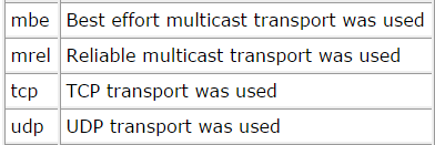
Some filenames include an indication of the transport and message size used in the test results being reported. The message size is a number indicating the number of payload bytes added to transmitted samples. Sizes used include: 50, 100, 250, 500, 1000, 2500, 5000, 8000, 16000, and 32000 bytes. The transport is indicated by one of the following abbreviations:

The latency plot script file names include a type indication that determines if latency or jitter is plotted. These correspond to the plot script files supplied as part of the OpenDDS-Bench framework, but differ in that these files only produce a local chart and do not create an image file for the charts The files and scripts included are summarized in the table below.

File(s)	Contents	Description
data/latency--.gpd	Data set of sample measurements and derived values.	These files contain the full set of latency and jitter data for each test case. Tests are executed for different transport and message size combinations. The resulting data is then converted into these files which contain several GNUPlot format indexes. The data consists of: Index Column 1 2 0 latency measurements derived jitter data 1 lowest value of bin latency sample count in bin 2 lowest value of bin jitter sample count in bin 3 latency quantile data --- 4 jitter quantile data ---
data/throughput-data.gpd	Throughput data for tests.	This file contains the summary data for the execution of the steepest ascent test cases for Throughput tests using the UDP transport. The Bidirectional and Publication Bound Throughput tests each have a separate index with the message rate, sample size, and measured throughput included as column data: Index Column 1 2 3 0 sample sending rate (samples/second) sample size (bytes/sample) Bidirectional Throughput Test measured throughput (bps) 1 sample sending rate (samples/second) sample size (bytes/sample) Publication Bound Throughput Test measured throughput (bps)
data/latency.csv	Summary data for all tests.	This file contains a summary of all the statistical estimates for each transport and size combination for which test data exists. This data is in the form of a CSV file with fields defined as described in the file itself. The statistics include the arithmetic mean and standard deviation, the median and MAD, and the maximum and minimum values measured. This data is used to produce the summary charts for both latency and jitter.
data/latency--.stats	GNUPlot loadable string variables.	These files contain GNUPlot specific commands to load string variables containing the statistical summary data for the particular transport and size of the file. The string variables are: latency_stats which is added as a label to the latency histogram chart; and jitter_stats which is added as a label to the jitter histogram chart.
scripts/plot--summary.gpi	GNUPlot commands to create a summary chart.	These commands will produce a chart containing the summary data for each transport at all measured message sizes.
scripts/plot--timeline.gpi	GNUPlot commands to create a timeline chart.	These commands will produce a timeline chart containing the individual sample data plotted over time.
scripts/plot--quantiles.gpi	GNUPlot commands to create a quantile chart.	These commands will produce a quantile chart containing individual sample data.
scripts/plot--histogram.gpi	GNUPlot commands to create a histogram chart.	These commands will produce a histogram chart of the latency or jitter data.
scripts/plot--density.gpi	GNUPlot commands to create a density chart.	These commands will produce a kernel density estimation chart of the latency or jitter data.
scripts/plot-throughput.gpi	GNUPlot commands to create a throughput results chart.	These commands will produce a plot with the results from the throughput test cases in the throughput datafile.

Data and Script files included in the article code archive

Latency and Jitter

The Latency and Jitter data collected from the preconfigured Latency tests of the OpenDDS-Bench framework can be summarized and charted in different forms. This includes summary plots of the entire data set, Timeline plots for individual test runs, Quantile plots, Histograms, and Density plots for both the measured latencies and the jitter.

• Summary Plots
  

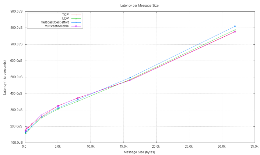
  The entire data set of measured latency data can be summarized in a single chart. The preconfigured tests measure latency for each of the transport implementations passing messages of 10 different sizes. The median value for each test's latency is plotted as a point on this chart and the data points for each transport type are connected.

  The following plot shows the measured latency data collected in a test performed in our lab environment. The linearity of the plot demonstrates that the latency delay per bit is constant as the message size is increased. Since the message size is included in the delay measurement, this is expected. The point at which the 0 x-axis value is reached shows the processing overhead for the test independent of any message bits.

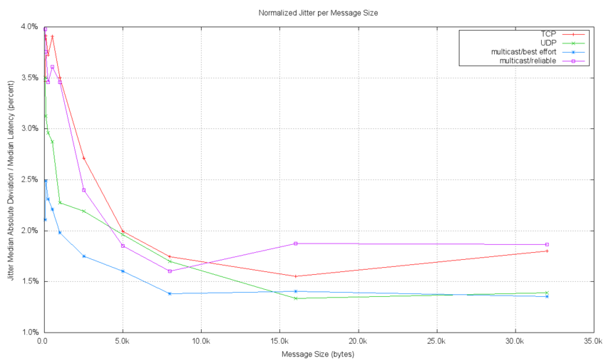
The Jitter data is also summarized for all transport types and each message size as well. Jitter is best described in a normalized fashion. This means that the jitter is presented relative to the latency value at the point the jitter is measured. This allows comparisons of jitter performance at different message sizes to be meaningful. The following plot shows the jitter as a percentage of the latency at the message size where the measurement was taken. This data corresponds to the latency data shown in the previous plot.

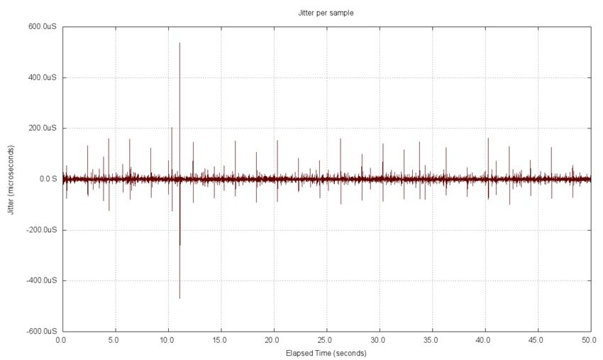
• Timeline Plot
  
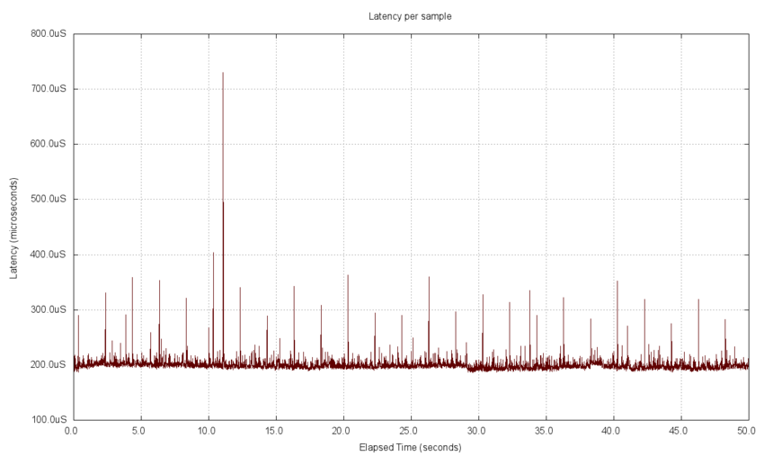
  A timeline plot shows each measured data point over the duration of the measurements. The preconfigured tests capture and report the last 5,000 samples sent during testing. The latency measurements are shown below. Periodic noise can be seen in these plots, with one spike at about 11 seconds into the data set. The periodic noise is likely to be caused by other system processes that run regularly. The tests charted here were executed on a time shared workstation with a user desktop present and system services running. The chart clearly shows that the majority of the delays are in a narrow band at the low end of the measurement range with some noise components added, presumably by other system processing.

The jitter timeline plot is similar to the latency plot, but it has both positive and negative values included. The same noisy characteristics appear in the jitter plot as in the latency timeline plot. Presumably this is for similar reasons. Indeed the same period can be seen in the noise, and a similar spike at about 11 seconds into the data set correspond to those in the latency chart.

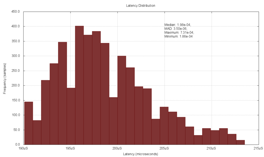
• Histogram Plot
  
  Histogram plots are simple bar charts that show an estimate of the probability density function for a population using the measured data. This is done by dividing the measurements (the latency delay or jitter here) into a series of bins and charting the number of measured data points in each bin interval. They are typically plotted as adjacent bars rather than points to indicate that the measurements fall within the range rather than at a single point within the range.
  
  It is common to choose the bin widths to be the same for the entire interval. It is also common to restrict the interval to where the majority of the data lies in order to provide additional detail for the majority of the measurements. This is done because a few extreme data measurements will result in many equal width bins containing no data measurements (0 values in the histogram), thereby reducing the information content of the chart. With a restricted range a few data points are not included, but the majority of bins will have meaningful (non-zero) data to plot.
  
  The following chart plots the latency delay data from above as a histogram, with 25 bins of equal width between the 5% and 95% measured values. 4,500 of the 5,000 data measurements are included in this plot. Note that even with the range restriction, the chart is only an estimate of the population probability density due to the details of the measurements, the bin number, and bin width. The shape can be seen to approximate a unimodal distribution with a peak at about the median value. Also note that the distribution is clearly not Normal as it is asymmetrically skewed towards the right.

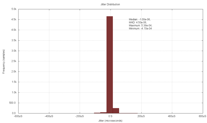
The following histogram of the jitter data includes all 5,000 measurements without a range restriction. It also includes 25 bins of equal width. It is clear that since there are a few outlier measurements (at the extremes) the bins which have visible amounts of data are just a few in the center of the plot. Excluding the extremes would allow more bins to contain measured data values and the shape of the density plot would be clearer. In this case the density appears as a peaked Normal distribution with tails to both sides, as expected.

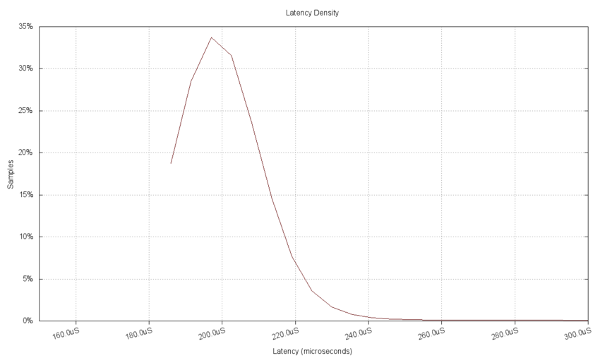
• Density Plot
  
  Kernel density estimation plots are a slightly more analytic method of providing probability density estimates for a population using the measured data. This is done by replacing each measurement with a location (mean) of the measurement and a spread (deviation) selected by a free bandwidth parameter. Then the entire data set is summed and normalized by the number of measurements included
  
  More spread out estimates (larger bandwidth) will result in a smoother resulting plot while narrower estimates (smaller bandwidth) will be less smooth. The plotting scripts provided use a common bandwidth parameter for the entire data set. It is possible to select a different bandwidth for each data point, but this is more useful for multivariate distributions rather than our single measurement charts.
  
  The following chart of the latency delays using a Gaussian estimation kernel with a bandwidth of 10μS shows more clearly the non-Normal distribution and asymmetry when compared with the previous histogram of the same data. Also note that even though the aggregate estimate (sum of individual measurement estimators) will have values outside of the original extreme measurement ranges, the plot is truncated at those extreme values to clearly indicate where the range of measurements terminated. This is clearest on the low side of the chart where no data is plotted for delays below the minimum.

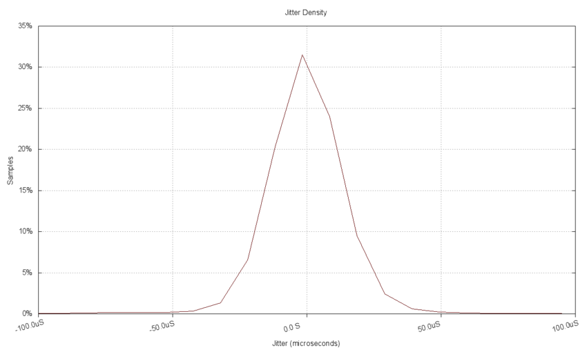
The following chart of the delay jitter uses the same kernel estimator as for the latency data above. It shows the same peaked Normal distribution seen in the histogram. No data was excluded from the estimate, although the visual range of the chart was reduced to the center portion for clarity. The range restriction here affects the plot view only, there is no difference to the plotted data due to the limited range as there was in the binned histogram.

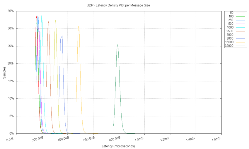
The following chart aggregates the results of kernel density estimation for measurements from 10 separate tests. Each test clearly has a different peak value. This chart allows the latency delay performance for each message size test to be compared quickly.

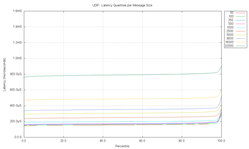
• Quantile Plot
  
  Quantile plots represent a cumulative distribution function for a set of measurements, but in a non-traditional format. A typical distribution function will plot the probability of a measurement being less than a value. A quantile plot charts the maximum value for given probability. This effectively flips the axes of the chart. For the measured data set the probability is taken as the portion of the measured data.
  
  In general the shape of the quantile plot can be used to infer information about the measurements. An almost horizontal line would indicate a very narrow distribution about the mean with no extreme values. If extreme values occur, to either the high or low end, they would appear as tails on the chart. If there were different realms of operation that were being measured, then segments for each realm would be apparent. For example if the latency measurements included both a direct and queued mode of operation, then the portion of operation using the direct mechanism would appear as a line segment with lower latency and the queued operation would appear with a larger delay. The slope of the queued operation line might then indicate the rate of queue growth during that mode of operation. The relative amount of time spent in each operating mode would correspond to the length of the different horizontal segments.
  
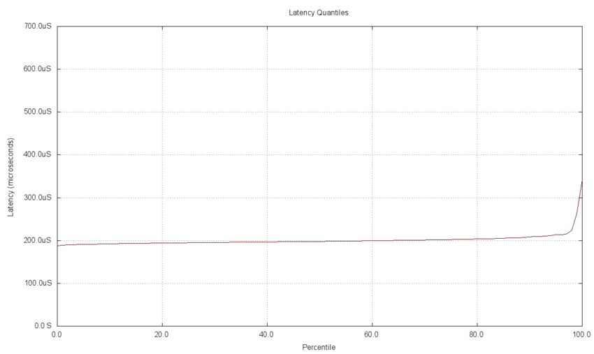
  The 5,000 measured latency delays are plotted in a quantile chart below. The flat horizontal line indicates that for the majority (98%) of the measurements the delay was very close to the median. This means that the delays with periodic noise seen in the timeline plot above include about a 2% contribution from the noise while the majority of the delays are very close to the median.

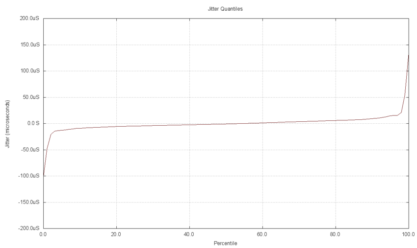
The jitter measurements for the data set are charted below. You can see that the jitter has a tail on both the low and high ends of the data. About 2% of the delay jitter is less than the middle portion (the low end tail) and 2% are greater than the higher portion (the high end tail). The majority of the jitter appears to be close to the median and centered on the zero axis.

The following chart aggregates the quantile plots for measurements from 10 separate tests. Each test clearly has a different median value. This chart allows the latency delay performance for each message size test to be compared quickly. For example, the slope of the line for each test and the point at which the tails form is seen to be consistent for all test cases.

THROUGHPUT

The OpenDDS-Bench framework preconfigured throughput tests include different test topologies, sample rates, and sample sizes. The throughput for each of these cases is extracted and can then be plotted. In addition to the measured throughput data it is typical to include the specified test bit rate and the network capacity on the chart to bound the test data. For tests with bit rates lower than the network capacity, the measured throughput is bounded by the specified rate. For specified bit rates higher than the capacity, the capacity bounds the measured throughput.

The network capacity is both theoretical and practical. The theoretical capacity is the rated network bandwidth, such as 100 Mbps or a Gigabit network with 1 Gbps capacity. The practical throughput can be estimated by using a typical transfer at maximum rate and measuring the achieved throughput. Transfers using the ftp protocol are commonly used to characterize practical limits on network usable bandwidth.

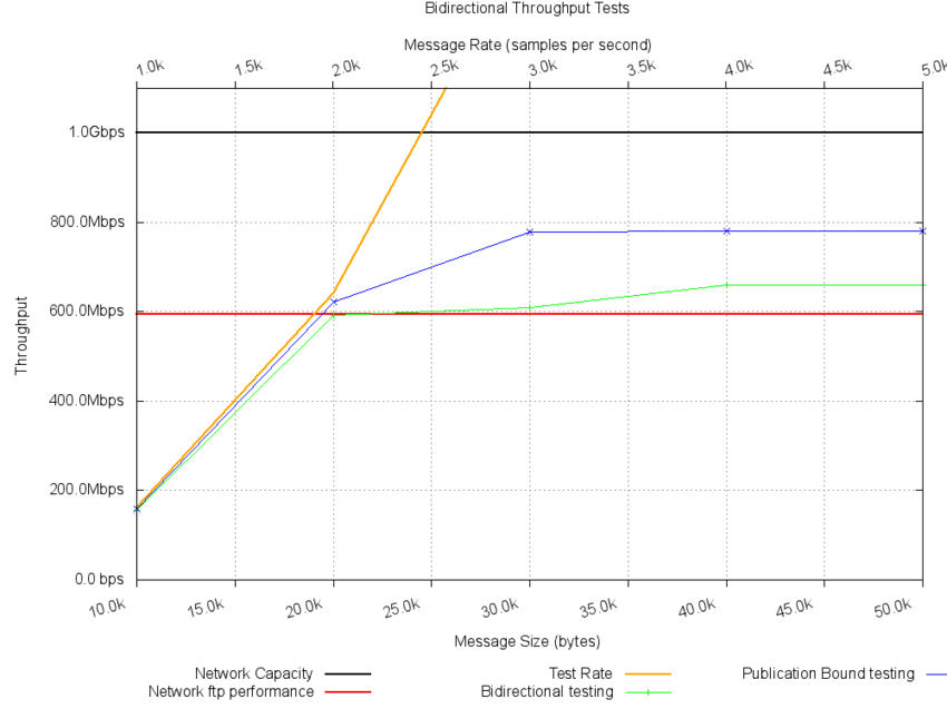
The following chart shows the results of two test topologies: bidirectional, and publication bound using a UDP transport implementation. They were executed in five separate test cases with different message rates and message sizes. The network was rated as a Gbps network, and the practical limit of the network was determined by transferring ftp data as fast as possible. The ftp performance was 595 Mbps, or just under 60% of the theoretical rated capacity.

The black horizontal line is the rated network capacity limit. The red horizontal line is the practical network capacity. The orange diagonal line is the specified test throughput. While this line is below the network capacity lines, it will bound the measured throughput. This is observed for both test topologies. Once the practical network capacity is reached, both tests then reach a throughput limit, one higher than the other. Since the bidirectional topology sends the message traffic from both the local and the remote host, they will collide as more traffic is added, resulting in dropped packets and the limit similar to the ftp protocol, which also includes back flow traffic. The publication bound test topology sends samples from the originating host to two separate terminating hosts. No traffic from the receiving hosts to the sending host is generated, which results in somewhat more of the theoretical bandwidth being used.

Summary

In this article we have discussed the various types of measurements taken for OpenDDS performance testing and evaluation. Issues with the measurements and their interpretation were touched on. A discussion of the ways to summarize the data as statistical values and as charts was undertaken. The charts that are available from the OpenDDS-Bench performance testing framework were identified and discussed. See theOpenDDS-Bench Users Guide^[2] for details on how to setup and execute the preconfigured tests. The framework also provides scripts to perform data reduction to the formats needed to produce the charts discussed in this article.

The knowledge of the chart types and what they represent will be valuable in reviewing the existing and future performance testing results for OpenDDS that will be published. OpenDDS users can generate these charts locally for target system environments. They can then evaluate and compare the various performance parameters applicable to the desired system operation. The example charts were generated from testing in a low performance desktop environment and should not be used as a basis for evaluation of OpenDDS. Users are encouraged to use the OpenDDS-Bench performance test framework on their own systems to evaluate OpenDDS for suitability.

References

• [1] OpenDDS Portal
  http://www.opendds.org
• [2] OpenDDS-Bench User Guide
  https://svn.dre.vanderbilt.edu/viewvc/DDS/trunk/performance-tests/Bench/doc/userguide.html?view=co
• [3] OpenDDS Subversion Repository
  https://svn.dre.vanderbilt.edu/viewvc/DDS/trunk
• [4] Article Code Archive
   http://www.ociweb.com/mnb/code/mnb201003-code.tar.gz
• [5] GNUPlot
  http://gnuplot.info/ 
• [6] Binary Prefixes
  http://en.wikipedia.org/wiki/Binary_prefix 
• [7]Summary Statistics
  http://en.wikipedia.org/wiki/Summary_statistics 
• [8] Robust Statistics
  http://en.wikipedia.org/wiki/Robust_statistics 
• [9] Random Variable Sum
  http://en.wikipedia.org/wiki/Sum_of_normally_distributed_random_variables 
• [10] Dispersion
  http://en.wikipedia.org/wiki/Statistical_dispersion 
• [11] Robust Scale 
  http://en.wikipedia.org/wiki/Robust_measures_of_scale 
• [12] Median Absolute Deviation
  http://en.wikipedia.org/wiki/Median_absolute_deviation
• [13] Kernel Density Estimation
  http://en.wikipedia.org/wiki/Kernel_density_estimation
• [14] Quantiles
  http://en.wikipedia.org/wiki/Quantiles
• [15] Packet Delay Variation
  http://en.wikipedia.org/wiki/Packet_delay_variation
• [16] Jitter
  http://tools.ietf.org/html/rfc3393
• [17] Gaussian Distribution
  http://en.wikipedia.org/wiki/Gaussian_distribution
• [18] Rayleigh Distribution
  http://en.wikipedia.org/wiki/Rayleigh_distribution