Machine Learning in Practice: Using Artificial Intelligence to Read Analog Gauges
By Xiao Yang, OCI Director, Machine Learning
June 2019
Background
Visual inspection is necessary to obtain readings from analog gauges. In many industries, this means a human operator must travel to the gauge's location, read its current value, and log that value to enable the data to be used elsewhere.
The ability to read an analog gauge using computer vision allows for the integration of readings into an automated system, which stands to deliver significant advantages, including:
- Reducing the need for a maintenance crew to travel to remote locations
- Providing near real-time, continuous access to gauge levels
- Allowing for digital monitoring of gauge readings and automatic alerts when readings go out of tolerance
Project Description
The Deep Gauge project described in this article is designed to implement support for reading an analog gauge using computer vision and machine learning.
The objective is to train the system to read gauge values for use in commercial and industrial settings in order to minimize the need for manual inspection and intervention. Through the use of a mounted camera, a video feed can be processed via computer vision software and converted to a digital data stream. This digital data can then be monitored and logged for use within the organization.
One application of this capability is in the power industry, where many existing enclosures still utilize analog gauges that must be read by technicians, who must log the data for subsequent analysis.
Approach
Various approaches have been explored with image processing algorithms using tools like OpenCV. However, scaling these methods in large-scale industrial applications has been limited by an extensive, manual feature extraction process.
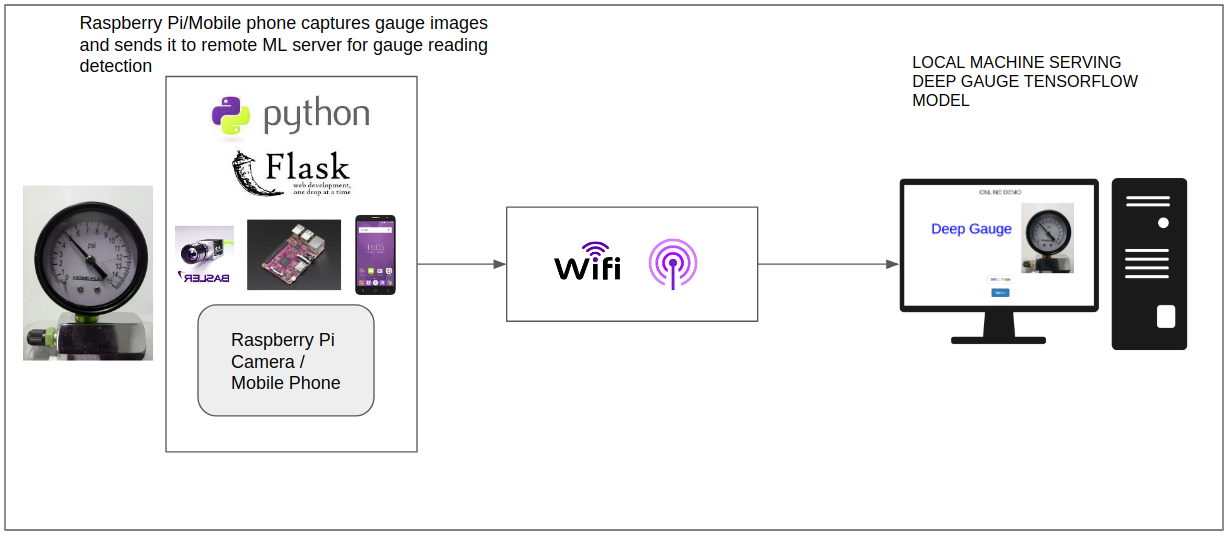
For this effort, we use a convolutional neural network (CNN) -based deep learning approach to read gauge dial readings, using the images captured from edge devices, such as phones and a Raspberry Pi. A TensorFlow custom estimator is used to train the CNN model on the Google Cloud Platform (GCP) ML Engine. The trained model is also deployed on GCP and employed to make predictions accessible via a standard RESTful interface.
Data Generation, Preprocessing, and the Data Pipeline
Dataset collection is an essential part of training deep learning models.
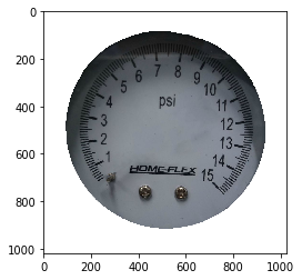
To train an effective model for this project, the dataset must contain images of a gauge dial at multiple needle positions. Manually creating gauge images for every position by physically manipulating the dial position is tedious and may be infeasible in many cases.
The approach for the Deep Gauge reader is to start with a gauge dial image in a single position and use OpenCV libraries to synthetically generate the image dataset with needle positions at different locations. The images are further augmented using scaling, rotation, zooming, translation, and cropping to obtain a sufficient dataset to train the model.
The block diagram below shows a process for generating a training set for a gauge dial in multiple dial positions.
You can access the code to perform these operations here.
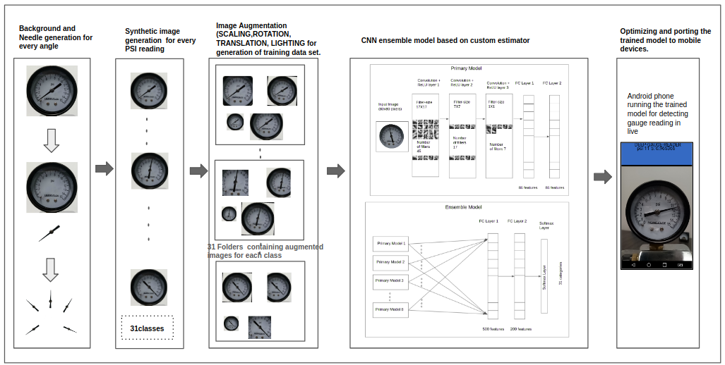
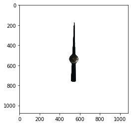
The needle for each individual image is separated from the background using an image processing tool. Once separated from the gauge dial, the needle image is rotated to each of the required angles and reconnected to the background to generate candidate images for every label/class corresponding to gauge dial reading.
Correct Needle Placement
- Determine what angle the needle needs to be set to in order to display at the 0 gauge number.
- Determine what angle the needle needs to be set to in order to display the 15 gauge reading.
- Iterate over the range between the 0 angle and the 15 angle
- Create the image with the labels in PSI instead of degrees.
Data Exploration: Image Data Preparation
The image dataset is first split into two subsets: "train" and "validation." The training dataset contains 1,315 images and the validation dataset contains 329 images.
The following code block shows how the datasets can be obtained via a LoadImg module.
# The color_mode is either 'rgb' or 'grayscale' (default).
X_train, X_validation, y_train, y_validation, cls_indices = LoadImg.Dataset.prep_datasets(
    ver_ratio=0.2, container_path='./data/ImageEveryUnit',
    final_img_width=79, final_img_height=79,
    color_mode="grayscale", random_state=1911)
Next, the images' size and color mode are adjusted using the keras.preprocessing package.
In this example, a width and height of 79 were chosen, so each image's shape is (79, 79, 3).
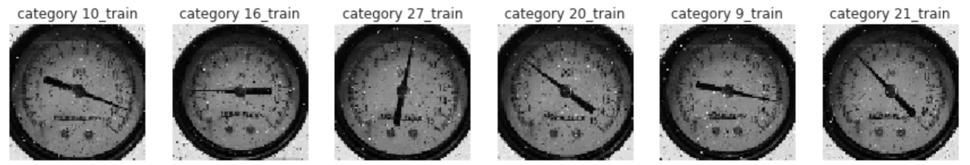
Then 12 images are randomly selected from the train dataset and 12 are selected from the validation dataset, as shown in these code blocks.
The following augmentation techniques are applied to each image of these 12 images to help the model generalize better for various conditions and minimize overfitting:
- Scaling
- Translation
- Rotation
- Adding salt-and-pepper noise
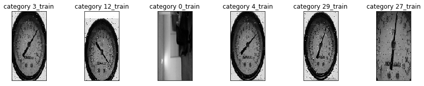
Training Data Samples
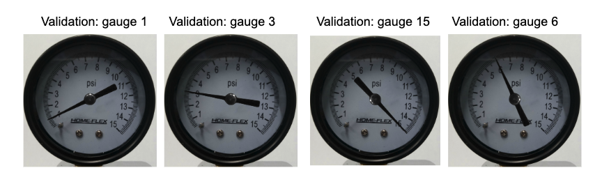
Validation Data Samples
Data exploration: Ensembling
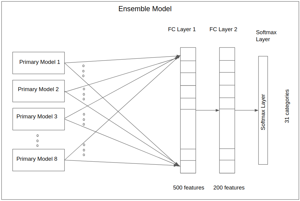
The objective of this work is to train multiple models (here, referred to as primary models) and eventually use them to construct an ensemble model (a two-layer, fully connected neural network) that can perform with higher validation accuracy than each individual primary model.
To construct the ensemble model, the primary models are trained first. Then the probabilities (i.e., the output of the last layer softmax activation functions) of all models are computed and stacked into an array (1D tensor). This array becomes the input for the ensembling deep neural network (DNN).
The ensemble DNN is a classifier that is to predict the same 31 categories. It is trained with the same training dataset, and its performance is evaluated against the same validation dataset used for the primary models.
Training the Primary Models
For each primary model, a CNN architecture is trained and used to predict the 31 gauge images categories:
- 30 categories that show the pressure levels collected by the gauge with half of the pressure unit (here psi) increments
- One NaN category
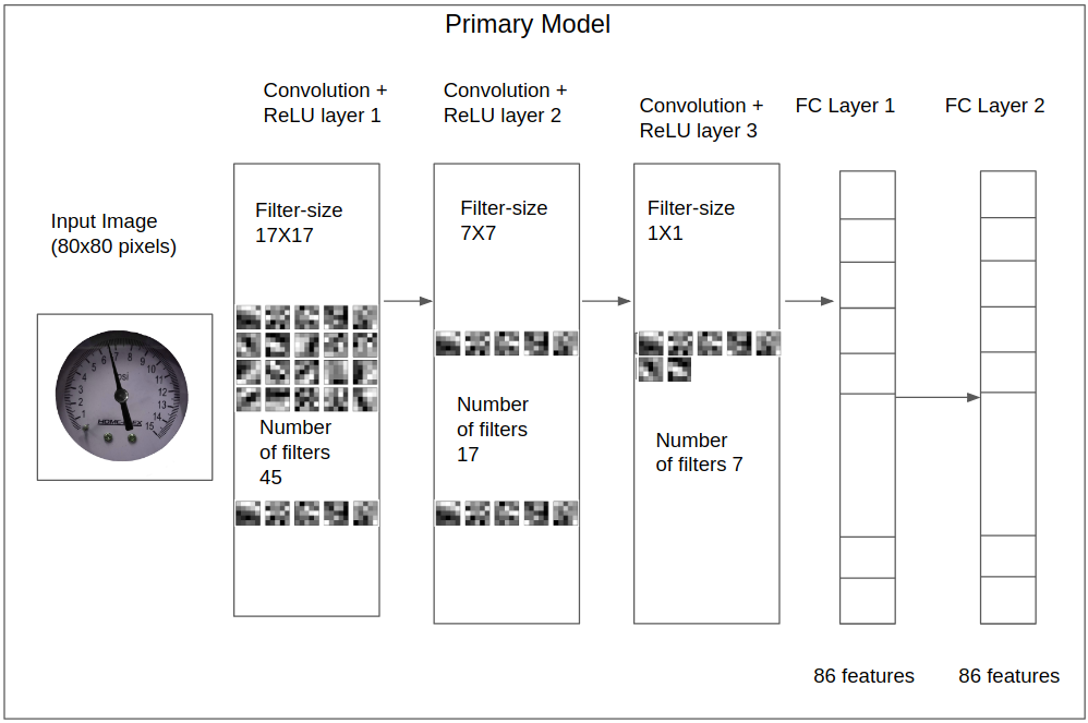
The CNN model consists of three CNN layers and two fully connected (FC) layers.
The layers are defined in the NewLayers module: CustomEstimator/modules/primary_models_modules/train_modules/NewLayers.py).
The CNN architecture is structured in the NeuralNet module: (CustomEstimator/modules/primary_models_modules/train_modules/NeuralNet.py.
The activation function of all layers is rectified linear unit (reLU), with the exception of the last layer, which is softmax.
The following diagram shows the primary model architecture.
TensorFlow Model: Primary Models
Deep Gauge uses eight models for detecting gauge readings accurately from gauge images. For each individual model, a CNN architecture is trained and used to predict 31 gauge image categories:
- 30 categories that show the pressure level collected by the gauge with half of the pressure unit (here psi) increments
- One NaN category
Hyperparameter Tuning the TensorFlow Primary Models
For the primary model hyperparameter tuning, a model is first trained using images with the same width:height ratio as the original images.
The hyperparameters of this model are manually tuned, and the ones that resulted in improved performance (i.e., validation dataset accuracy) are used for the subsequent primary models.
Feature Engineering
The layers are defined in the NewLayers module, modules/NewLayers.py and are combined in the NeuralNet module, modules/NeuralNet.py.
The activation function of all layers is ReLU, except for the last layer, which is softmax.
Training the TensorFlow Primary Models
To train the primary models, the cross-entropy function[1] and Adam algorithm[2] are employed as the cost function and optimizer, respectively.
Model performance is evaluated in each training iteration via the accuracy of the validation dataset, and the model checkpoint is saved in the modules/primary_models_modules/logs/models/main folder whenever accuracy is improved.
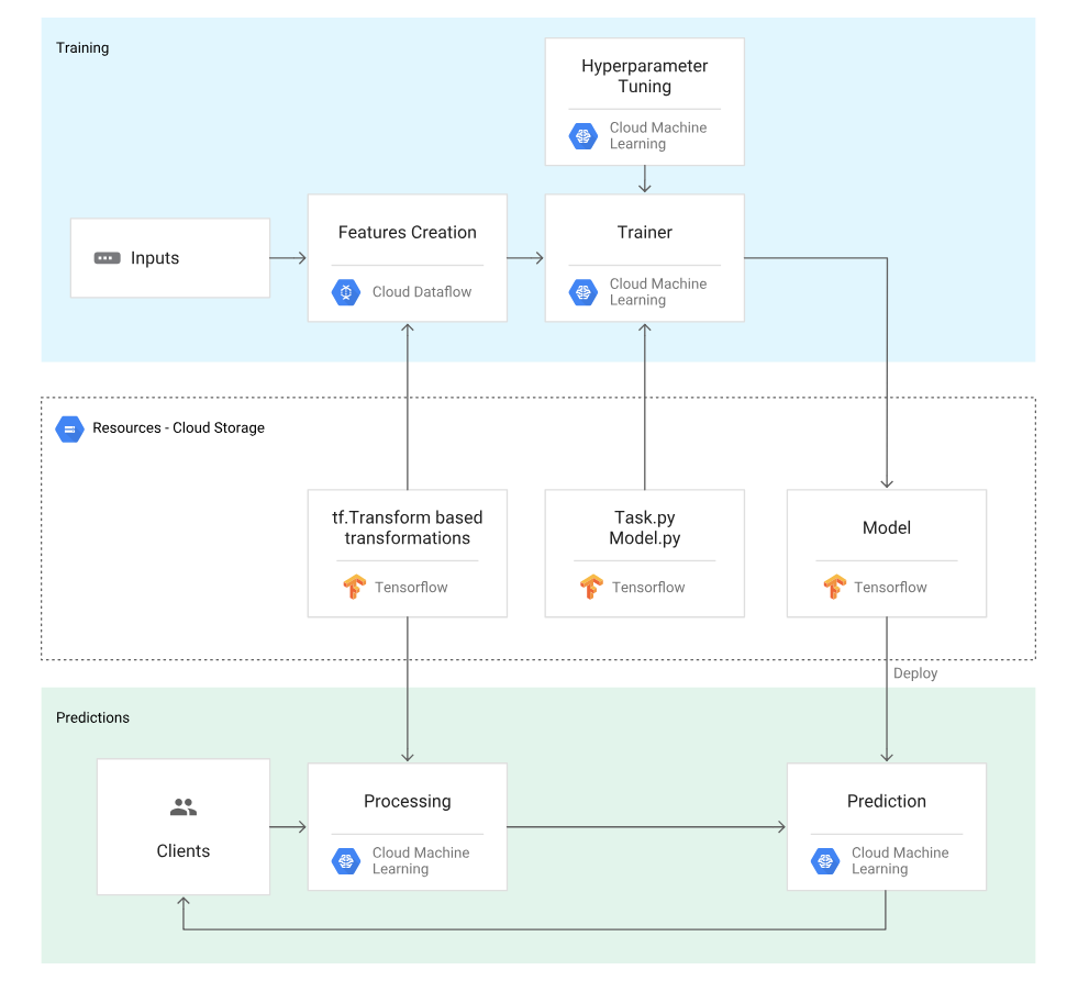
Training of Model in GCP Environment
TensorFlow Model: Ensembling
The objective of this work is to train multiple models and eventually use them to construct an ensemble model (here, a two-layer, fully connected neural network) that can perform with higher validation accuracy than each of the individual primary models.
To construct the ensemble model, the individual models are trained first. Then the logits (i.e., the output of the last layer softmax activation functions) of all models are computed and stacked into a numpy array (1D tensor). This array becomes the input for a two-layer, fully connected neural network.
The final neural network is a classifier that is to predict the same 31 categories. It is trained with the same training dataset, and its performance is evaluated against the same validation dataset used with the primary models.
TensorFlow Model: Custom Performance Metric
The validation dataset accuracy is used as the metric to evaluate model performance during model training, and the model checkpoint is saved whenever it increases.
In tie cases where the performance metric does not change over training iterations, if the median of the validation dataset's true label logits increases, the saved checkpoint is overwritten by the latest model checkpoint.
In addition to the model evaluation using the whole validation dataset accuracy, the model performance for each specific category is also evaluated using the following equation:
catPerf = (number of true predictions in validation dataset for that category)/(total number of validation samples for that category)
Whenever the catPerf increases during training, the model checkpoints are saved in folders corresponding to their categories (e.g., logs/models/psi_2).
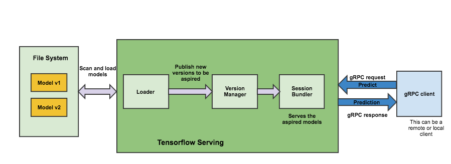
TensorFlow Model: Deployment
After training an Estimator model, we create a service from that model that takes requests and returns a result. We can run such a service locally on our machine or deploy it in the cloud.
TensorFlow Serving Using SavedModel with Estimators
To prepare a trained Estimator for serving, we export it in the standard SavedModel format as follows:
- Specify the output nodes and the corresponding APIs that can be served (Classify, Regress, or Predict).
- Export your model to the SavedModel format.
- Serve the model from a local server and request predictions.
ML Engine Deployment
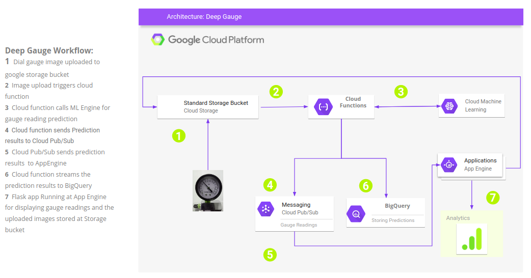
Cloud Functions: A set of GCP functions for writing, deploying, and triggering a Background Cloud Function with a Cloud Storage trigger.
gcloud components update &&
gcloud components install beta
gsutil mb gs://YOUR_TRIGGER_BUCKET_NAME
gsutil mb gs://ocideepgauge-images
gcloud functions deploy predict_gauge --source=. --runtime python37 --trigger-resource ocideepgauge-images --trigger-event google.storage.object.metadataUpdate
Cloud Pub/Sub: These are the Google Cloud CLI commands to create a topic, allowing messages to be published to the topic after the subscription is created and available to subscriber applications. This GCP module relays the message between user input and online prediction through the deployed ML model.
gcloud pubsub topics create my-topic
gcloud pubsub subscriptions create my-sub --topic my-topic
gcloud pubsub subscriptions create gauge-prediction --topic gauge-prediction
Online Prediction
For online prediction, a flask-based web app is developed that allows users to stream gauge images or upload gauge dial images to an ML engine hosting the Deep Gauge deep learning model. The gauge readings detected by the model are displayed in the user's browser.
Conclusion
We developed an end-to-end ML workflow with image recognition for analog gauge reading. We deployed it through Google Cloud Platform, which is readily served via many applications (mobile or desktop).
By custom training a deep neural network along with ensemble learning, we can achieve an overall accuracy of ~92%.
Here's what we learned through this journey:
- Deep learning can provide better predictive performance at scale over conventional imaging analysis, such as image segmentation based algorithms in OpenCV.
- The number of images available for certain categories is often limited for building deep learning models, and the data augmentation approach with synthetic image generation can effectively mitigate the small size problem while significantly improving model accuracy.
References
- [1] Ian Goodfellow, Yoshua Bengio, and Aaron Courville (2016). Deep Learning. MIT Press. Online
- [2] Diederik P. Kingma and Jimmy Lei Ba. (2014). Adam : A method for stochastic optimization. arXiv:1412.6980v9
Software Engineering Tech Trends (SETT) is a regular publication featuring emerging trends in software engineering.
