Extracting Value from Data
By Mike Martinez, OCI Principal Software Engineer
November 2015
Introduction
In this article, we present a model of how Big Data analytics works with an Industrial Internet of Things (IIoT) application. Our analysis revolves around a fictional gas station and convenience store chain, which we call Carmageddon.
Carmageddon represents a business that generates .
The business is made up of 700 gas stations in 20 cities, with a total of 7,000 gas pumps and 2,000 fuel tanks that have been acquired over time.
Our model simulates Carmageddon's operations.
Carmageddon is currently struggling with issues with:
- EPA compliance
- Climbing preventive maintenance costs
- Frequent outages due to breakdowns within their aging pump and tank infrastructure
A failed pump costs approximately $3K per day or $1M per year; an empty tank costs (in lost revenue) $7K per day or $2.5M per year.
Carmageddon's current approach to dealing with pump and tank failures is reactive. They would like to develop a strategy and approach that enables them to be proactive in preventing sales and revenue losses.
The proposed solution is to develop an IIoT ecosystem, which takes advantage of sensors that collect data from Carmageddon's pumps and tanks and stream data to a cloud-based analytics engine, which predicts tank and pump failures and thereby empowers the business to avoid unexpected failures and losses in revenue.
This solution is demonstrated and may be viewed at: http://carma.demo.ociweb.com/.
In this article we will describe the analytics involved in establishing a maintenance interval for the fuel pumps. This solution minimizes the total cost of repairs within the context of a system that uses cloud-based processing to gather and ingest large amounts of data, present them in a useful fashion, and utilize analytic methods to generate value from the gathered data.
What follows includes a quick exploration of failure models, with the selection of a likely candidate for our model.
After that we generate some synthetic test data using the theoretical model, which will allow us to evaluate our data analysis processing. We will create an analysis mechanism that allows us to estimate model parameters given only data that we can actually collect. The simulated data is then applied to the parameter estimation mechanisms to evaluate their performance.
Once we have a model, simulated data for that model, and a processing mechanism that allows us to estimate the model parameters from measurable data, we will explore how we can use the model to predict equipment failures and how these predictions can be used to reduce the cost of failures in the corporation. This involves evaluating the different contributions to costs for failures and determining how to select a maintenance interval reducing these costs to an overall minimum.
Overview
The first step is to derive a suitable model that determines when the simulated pumps will fail.
Next, we process our simulated data with the date of inception – when the pumps were new or last repaired – and the age at which they will fail.
From there, we illustrate how the model parameters are estimated from data and show the accuracy of this estimation process using the generated simulation data.
Once we have the model and derived parameters from the simulated data, we determine the maintenance costs for repairing the pumps.
Note that we are identifying the minimum maintenance costs (by looking at data regarding maintenance costs at different maintenance intervals) and proactively scheduling maintenance (as opposed to reacting to the actual breakdowns). This effectively reduces the amount of data that we have for estimating the parameters. Therefore, once we start the new maintenance intervals, we will need to spend a greater amount of time before reaching the same confidence in our estimated parameters.
Once we have examined the costs without using scheduled maintenance and then optimized the interval for scheduled maintenance, we obtain results that show a positive value for implementing the scheduled maintenance:
- Implementing scheduled maintenance results in a savings of 43.6% (costs are 56.4% of the base case).
- Implementing scheduled maintenance saves $1,052.48 per pump annually, or $7.4M for the corporation.
After we obtain these results, we discuss some of the issues that might arise, as well as some cautions about use of the model and subsequent parameter estimation.
Fuel Pump Reliability
In order to determine maintenance costs for the fuel pumps, the reliability of the pumps must be modeled. Since this is a demonstration project, we can make many simplifying assumptions without losing the ability to illustrate the techniques involved in doing this.
Some conditions that we ignore include the specifics of how failures occur. We can also characterize the types of failure as an aggregate average cost for maintenance actions, rather than attempting to identify each failure case or repair result. We can also lump all of the different component lifetimes into a single time-to-failure value that represents the aggregate average over all of the components.
Pump Survival
Pump survival to a specific age is defined as the probability that a pump has not failed when it achieves that age. Each pump fails with a probability defined by a probability density function (PDF) characteristic of the pumps. Using different density functions results in different survival curves for the pumps.
Modeling pump failures consists of assigning an initial age (date of installation or repair) to each pump, then determining failure points using the model.
Note that, once a model has been selected, processing of the inbound actual data consists of estimating the model parameters from the observed data. Predictions can then be made using the model with the best-fit parameters.
We consider two models here:
- A constant hazard rate model
- A log-normal failure rate model
Using R code to perform the modeling and simulation for this analysis, we start by setting up some useful values to be used. Among the variables we create include a mean time to failure (MTTF) value and a volatility estimate, which anticipates the model that we might use.
MTTF is a common way to express the average time we expect will elapse before a product fails. That is, half of the failures will occur before this time, and half will occur after this time. It does not constrain the actual shape of the failures over time in any way.
The volatility estimate is a mechanism that we can use to indicate how much randomness is included in the failures. That is, a higher volatility allows a model to include failures that clump together more often that a model with lower volatility. This value will be applied differently for different models.
- # Repeatability
- random_seed <- 2112
- set.seed(random_seed)
-
- # Plotting X variable (months)
- grid <- seq(0,40,0.1)
-
- # Probability scale values
- quantiles <- seq(0,1,by=0.01)
-
- # Corporation parameters
- annual_revenue <- 2000000000
- population <- 7000
-
- # Modeled time to failure and variability
- mttf <- 34
- exp_sigma <- 1.2
-
- # Additional useful values
- current_time <- Sys.time()
- epoch='1970-1-1'
- seconds_per_day <- 24 * 60 * 60
- days_per_year <- 365
- months_per_year <- 12
- days_per_month <- round(days_per_year/months_per_year)
Failure rate models can be simple or complex. We opt for a model that is as simple as possible, while still useful. For complex products, failure rates can be created by combining failure models for smaller, simpler elements of those products. This results in very complex failure models for these products. If we accept some margin, between what a model predicts and how failures may actually occur, more simple failure models may be used to approximate more complex models.
A common failure rate model frequently used is the bathtub failure rate model. This model includes a high failure rate early in the life of a product, followed by a long period with a relatively low failure rate, then an increasing failure rate at what is referred to as end-of-life.
For our model, we simplify by assuming the high early failure rate is not present due to the suppliers performing “burn-in” testing. This kind of testing is specifically designed to weed out products that will fail early. What remains is a long period with a low failure rate followed by increasing failures at the end of the products lifetime.
Failure rate models have several interesting properties associated with them, including:
| Probability density function | the probability that a single failure will occur at a specific time (age) |
| Cumulative density function | the proportion of a population that will fail up to a specific time |
| Survival function | the proportion of a population that will not fail up to a specific time |
| Hazard function | the probability that a single failure will occur in the surviving population at a specific time |
We will consider two models here.
- The first is the constant hazard rate model, which is a common failure model used to estimate how long a product will last.
- The second is a log-normal failure model, which has a low failure rate followed by a period where the rate increases steeply.
Constant Hazard Rate Model
The simplest failure density function is the constant hazard rate, where survival is characterized by the exponential density function. This failure rate density function includes the MTTF value, but does not include any allowance for volatility.
\[\begin{aligned} (1)\quad & f(t) = \lambda \mathrm{e}^{-\lambda t} & \quad\text{Probability density function} \\ (2)\quad & F(t) = 1 - \mathrm{e}^{-\lambda t} & \quad\text{Cumulative density function} \\ (3)\quad & S(t) = 1 - F(t) = \mathrm{e}^{-\lambda t} & \quad\text{Survival function} \\ (4)\quad & h(t) = \frac{f(t)}{S(t)} = \lambda & \quad\text{Hazard function} \\ \end{aligned}\]
- exp_rate <- log(1/2)/mttf
- pexp_working <- exp( exp_rate * grid)
A survival curve for this density function appears as:
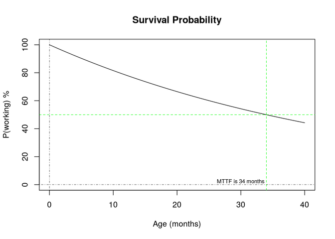
We expect fuel pumps to last for a time, then fail predominantly after they reach an age where components begin to wear out. The constant hazard rate model assumes that failures occur throughout the product lifetime at a regular rate.
Clearly the constant hazard rate model does not reflect the expected failure behaviors for the pumps.
Log-Normal Failure Rate Model
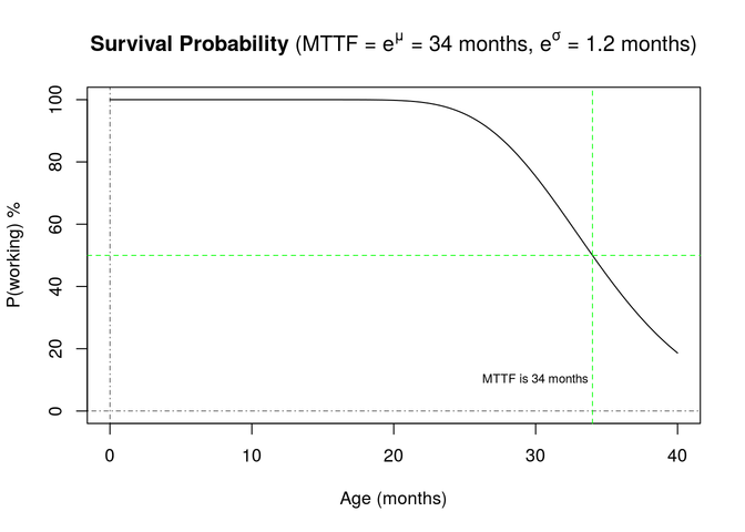
The log-normal probability distribution may be used to create a failure rate model that more closely resembles the right side of the typical failure rate “bathtub” characteristic curve describing hardware failures. The relevant formulas describing the model include:
\[\begin{aligned} (5)\quad & f(t) = \frac{\phi \left(\frac{\mathrm{ln}(t) - \mu}{\sigma} \right)}{ \sigma t } & \quad\text{Probability density function} \\ (6)\quad & F(t) = \Phi \left( \frac{\mathrm{ln}(t) - \mu}{\sigma} \right) & \quad\text{Cumulative density function} \\ (7)\quad & S(t) = 1 - F(t) = 1 - \Phi \left( \frac{\mathrm{ln}(t) - \mu}{\sigma} \right) & \quad\text{Survival function} \\ (8)\quad & h(t) = \frac{f(t)}{S(t)} = \frac{ \phi \left( \frac{ \mathrm{ln}(t) - \mu }{ \sigma} \right) }{ \sigma t \left[ 1 - \Phi \left( \frac{\mathrm{ln}(t) - \mu}{\sigma} \right) \right] } & \quad\text{Hazard function} \\ \end{aligned}\]
where
\[\begin{aligned} (9)\quad & \phi(u) = \frac{1}{\sqrt{2\pi}} \, \mathrm{e}^{^{-u^2}/_2} & \quad\text{Standard normal probability density function} \\ (10)\quad & \Phi(u) = \int\limits_{-\infty}^u \phi(z)\,\mathrm{d}z & \quad\text{Standard normal cumulative density function} \\ \end{aligned}\]
Modeling the survival function uses the log transformed variables:
- # log-normal distribution with mu of 34 months, standard deviation of 1.2 months.
- mu <- log(mttf)
- sigma <- log(exp_sigma)
-
- survival <- function(mu,sigma) { plnorm( grid, mu, sigma, lower=F) }
- ln_hazard <- function(mu,sigma) { dlnorm( grid, mu, sigma) / survival(mu,sigma) }
The hazard function can be derived as the ratio of the failure probability to the survival probability. This function may be used to understand the probability of failure at a particular age. It represents the probability that a pump that has survived to an age will then fail at that age.
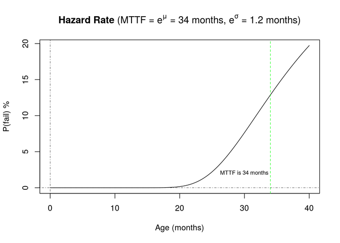
The hazard rate in this case is the tail end of the typical bathtub curve expected for pumps. If we assume the early failures are not present due to burn-in prior to purchase, the log-normal model is suitable for modeling the pump failures.
The log-normal density function results in a survival curve that more closely resembles actual failure characteristics:
Generating Simulated Failures
As part of the demonstration, we need to generate simulated failures. We use these simulated failures to test the parameter estimation formulas that derive the parameters from data.
Simulating the hardware failures consists of identifying the inception date for each pump, then projecting the age that each pump will fail. The inception date is the date the pump is “new,” that is, the starting point of the aging calculations.
Simulating Age at Failure
We can generate a simulated age at failure for all of our pumps using random variates from the log-normal distribution. To find each pump's age at the first failure, we generate one random value for each of the pumps:
- fail_times <- rlnorm(population,mu,sigma)
Sorting these ages and plotting the portion of surviving population against the age at failure results in the following chart:
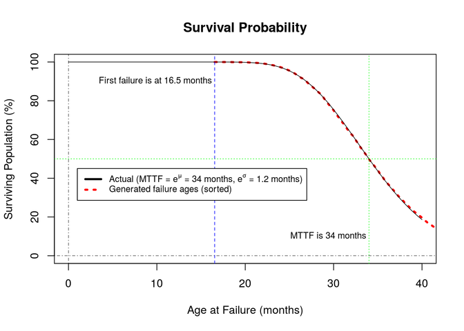
Note that this generated simulation data resembles the theoretical survival curve very well. We are confident that age at failure is generated correctly.
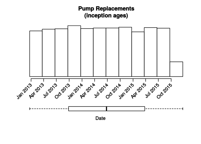
Assigning Inception Dates
The inception date for each pump is simulated as if each pump was last replaced at a random time in relation to any other pump. This will be done by allowing the inception date for a pump range from MTTF months prior to now, up to now.
For any pump that fails prior to now, the inception date is moved to that failure date, and a new age to failure is generated. This results in random ages for all of the pumps.
The date of a simulated failure is the sum of the inception date and the age to failure. Since this procedure utilizes the age at failure, to possibly adjust the inception date, these dates are derived after the age at failure data is available.
- inception_age <- runif(population,0,mttf*days_per_month)
- inception_dates <- as.POSIXct(current_time - seconds_per_day*inception_age,origin=epoch)
- inception_range <- range(inception_dates)
- inception_quarters <- seq(inception_range[1],inception_range[2],by="quarter")
The following histogram illustrates the distribution of inception times for the population prior to adjusting for failures earlier than now. The boxplot at the bottom shows that the distribution is uniform across the entire time period.
Estimating Model Parameters
Once we have simulated data, we can use that as input data to simulate actual measurements and determine if we will be able to estimate the model parameters closely enough to be useful.
Parameter Estimation Formulas
Estimating the actual parameter values for the log-normal model from measured sample data will be done using a maximum likelihood estimator for each of the two parameters. We will estimate the location (\(\hat{\mu}\)) and spread (\(\hat{\sigma}\)) parameters for the model. The exponentiation of these parameters is measured in time and can be used to characterise the age at failure for the pumps.
The values that are being used as input to the estimation formulas are the age at failure for each detected failure. This is the time at which a failure was detected to occur minus the time where the pump was considered "new". A pump is considered to be "new" when it is either replaced or repaired.
\[\begin{aligned} (11)\quad & \hat{\mu} = \frac{1}{n} \displaystyle\sum_{k=0}^n \mathrm{ln}(t_{fail,k} - t_{0,k}) & \quad\text{location estimation} \\ (12)\quad & \hat{\sigma} = \sqrt { \frac{1}{n} \displaystyle\sum_{k=0}^n \big( \mathrm{ln}(t_{fail,k} - t_{0,k}) - \hat{\mu} \big)^2 } & \quad\text{spread estimation} \\ \end{aligned}\]
Note that the input data to these estimation formulas are not directly available from actual input data. The simulated data provides this information directly.
When receiving actual measurement data, failures need to be detected first. This will be done by applying a threshold to the amount of time between sensor readings and when a reading has not been received from a sensor within this time, the associated pump will be considered to have failed. Once a failure has been detected in this way, then the inception age (last repair or replace date) will be subtracted from the current date, when the failure was detected, and the result used as the age at failure in the parameter estimation formulas.
Parameter Estimation Performance
We examine the estimated values of the parameters, referenced back to the non-log-normal values for generated simulation data. To do so, we generate a rolling window of the observed input data for the parameters as the data is received. This gives an intuition of how the values will behave when collecting actual measurement data.
- library(zoo)
- window <- 50
- rolling_mu <- exp(rollapply(fail_times,window,estimate_mu,partial=T))
- rolling_sigma <- exp(rollapply(fail_times,window,estimate_sigma,partial=T))
-
- mu_range <- range(rolling_mu)
- max_mu <- mu_range[2]
- min_mu <- mu_range[1]
- mu_error <- max(abs(mu_range-mttf))
-
- sigma_range <- range(rolling_sigma)
- max_sigma <- sigma_range[2]
- min_sigma <- sigma_range[1]
- var_error <- max(abs(sigma_range-exp(sigma)))
-
- model_conditions <- matrix(
- c( log(mttf), log(max_mu), log(max_mu), log(min_mu), log(min_mu),
- sigma, log(max_sigma), log(min_sigma), log(max_sigma), log(min_sigma)),
- ncol = 2
- )
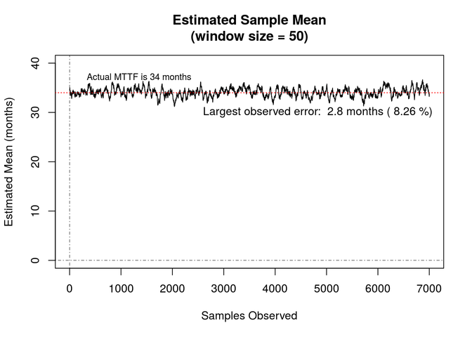
The plot below shows the estimated mu parameter value (translated back into months) over the first 7,000 generated data points using a 50 sample window. During this time, the estimate ranges from a low of 31.2 to a high of 36.7 months. The largest error from the actual value is 2.81 (8.26%) months.
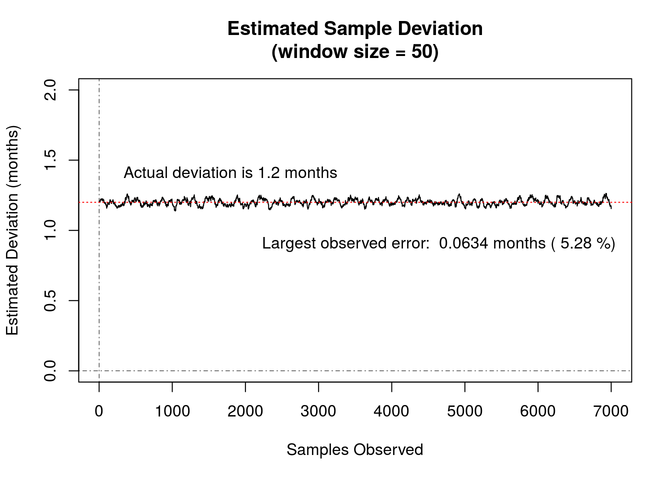
The plot below shows the estimated sigma parameter value (translated back into months) over the first 7,000 generated data points using a 50 sample window. During this time, the estimate ranges from a low of 1.14 to a high of 1.26 months. The largest error from the actual value is 0.0634 (5.28%) months.
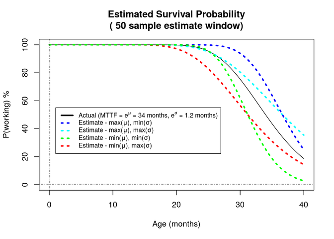
Comparing the survival curve of the actual age profile with the profiles derived from the estimated parameters, we can see in the chart below that the shape of the survival curve fits well, and the estimation errors bound the derived curve such that the actual curve lies within the estimated ones.
Predictions Using the Model
Now that we have confidence in the simulation data, and the processes used to generate it, we can use the parameters estimated from that data to make some predictions.
The obvious useful prediction to make would be to estimate the age at failure, which the log-normal model estimates. So once we have the model parameters, we can estimate when pumps will fail and perform preventative maintenance, such as replacing aging pumps, prior to the actual failure.
To utilize the prediction model for the age at which pumps will fail, we will determine the costs of repairing or replacing the pumps. Then we will find when to schedule maintenance so that the total maintenance cost is minimized.
The maintenance interval is the independent variable that we optimize using the cost as the metric. The optimal value is the desired maintenance interval, and the cost of performing maintenance at that interval will result in the lowest achievable cost.
Once we select a maintenance interval, we can determine the per pump cost for the maintenance and compare that to the case where we do no scheduled maintenance. This will allow us to determine if, and if so by how much, scheduling maintenance on the pumps will reduce overall costs.
When we schedule maintenance for pumps at a certain age, it is likely that some of the pumps will fail prior to this scheduled time. There will be no reduction in costs for these pumps. Likewise there will be no increase in their maintenance cost either.
Also, preventative maintenance prior to an actual failure will result in useful life of replaced components not being utilized, which is a cost as well. These costs must be balanced by any gains realized through scheduled maintenance compared to unscheduled, emergency, repairs.
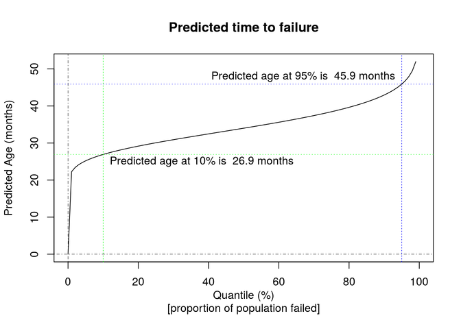
To start the prediction process, we can observe the model characteristic that allows us to determine the age at which a proportion of the entire population, or quantile, will have failed. This is the inverse of the cumulative probability function:
\[\begin{aligned} (13)\quad & t = F^{-1}(q) & \quad\text{Inverse cumulative density function} \\ \end{aligned}\]
Using this formula allows us to determine the age to schedule preventative maintenance, allowing a known portion of pumps to fail prior to this interval. The x-axis in the chart below is the quantile, or proportion of failed pumps, for which we are finding the predicted age.
- # Bind the model parameter estimates to the predictions.
- prediction <- function(q) { qlnorm(q, mu, sigma) }
Maintenance Costs
In order to determine when to schedule maintenance actions, we consider the costs for pump maintenance. Once we determine the total cost of maintenance actions at various maintenance intervals, we minimize the cost to find the interval for scheduling the maintenance actions.
To determine the cost of an individual repair, we find the average of all costs over the entire pump population. Costs to consider include: cost to repair or replace a pump, loss of revenue from a pump that is being repaired, and the loss from not utilizing the pump's full lifetime by repairing or replacing the pump before it fails.
It may be simpler to understand the cost components by analogy.
The predictions made here are similar to scheduling tire replacement. The mileage on any given tire is specific to that tire – tires are replaced as necessary and not as a group; this is similar to the age at which we perform maintenance on the pumps.
If we wait until the pumps fail, that corresponds to not replacing a tire until it goes flat. Clearly not a desirable outcome. If we schedule a tire to be replaced at a particular mileage, that corresponds to performing scheduled maintenance at a certain pump age. The cost of replacing a tire includes the cost of the replacement tire, plus labor costs, plus loss of use of the tire while it is being replaced. For the tire, loss of use is represented by miles not driven by the tire; for the pump, the loss is the time between when a repair or replacement was performed, and when the pump would have failed on its own (without maintenance).
- \(C_{\mathrm{pump}} \, = \, \$2,000.00 \,\) – cost of a new pump (replacement cost)
If a maintenance action requires a pump replacement, this is the maximum cost for the maintenance action.
- \(C_{\mathrm{repair}} \, = \, 60\% \, C_{\mathrm{pump}} \, = \, \$1,200.00\) – average non-replacement maintenance cost
This is the aggregate average over the entire pump population for the cost of maintenance that does not require pump replacement. This proportion holds for both scheduled and unscheduled maintenance actions.
- \(p_{\mathrm{replace}} \, = \, 20\%\) – proportion of maintenance actions that require the pump to be replaced
This is the proportion of all repairs that require pump replacement.
- \(p_{\mathrm{discount}} \, = \, 80\%\) – scheduled maintenance cost as a proportion of unscheduled maintenance costs
This is a reduction in maintenance costs due to the ability to leverage bulk supplier buying power andscheduled purchases, as well as the ability to schedule labor costs rather than paying a premium for unscheduled, emergency labor.
- \(mttr_{\mathrm{unscheduled}} \, = \, 7 \, \mathrm{days}\) – mean time to repair (MTTR) for unscheduled maintenance
This is the period of time that includes: pump failure, detection of pump failure, time to schedule and repair the pump, plus the time to return the pump to operation.
- \(mttr_{\mathrm{scheduled}} \, = \, 2 \, \mathrm{days}\) – mean time to repair (MTTR) for scheduled maintenance
This is the period of time that includes: start to completion of a scheduled maintenance plus the time to return the pump to operation.
Repair Costs
The cost of a repair for any pump will include the parts and labor for the repair. If the repair is done on a scheduled basis, then the cost should be adjusted to account for the shorter interval (on average) requiring more maintenance (on average) than would be incurred for repairs only performed on pumps which had failed.
<h3">Parts and Labor Costs
An unscheduled maintenance action cost will be the cost of a new pump times the number of new pumps needed, plus the cost of repair times the number of pumps repaired:
\[\begin{aligned} (14)\quad & C_{\mathrm{unscheduled}} = p_{\mathrm{replace}} \, C_{\mathrm{pump}} \, + \, ( 1 - p_{\mathrm{replace}} ) \, C_{\mathrm{repair}} & \quad\text{Cost of unscheduled maintenance action} \\ & = 0.2 \, \times \, $2,000.00 \, + 0.8 \, \times \, $1,200.00 & \\ & = $1,360.00 & \\ \end{aligned}\]
Scheduled maintenance costs are similar to the unscheduled costs, but have a lower cost for parts and labor:
\[\begin{aligned} (15)\quad & C_{\mathrm{scheduled}} = p_{\mathrm{discount}} \, C_{\mathrm{unscheduled}} & \quad\text{Cost of scheduled maintenance action} \\ & = 0.8 \, \times \, $1,360.00 & \\ & = $1,088.00 & \\ \end{aligned}\]
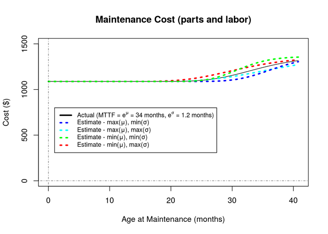
With these two repair costs available, the repair cost as a function of the quantile of failed pumps may be derived, and from there we calculate the repair cost as a function of the maintenance interval.
\[\begin{aligned} (16)\quad & C_{\mathrm{maintenance}} = q \, C_{\mathrm{unscheduled}} \, + \, ( 1 - q ) \, C_{\mathrm{scheduled}} & \quad\text{Cost of maintenance action} \\ & \, = F(t) \, C_{\mathrm{unscheduled}} \, + \, S(t) \, C_{\mathrm{scheduled}} & \\ & \, = C_{\mathrm{unscheduled}} \, \left( p_{\mathrm{discount}} \, + ( 1 - p_{\mathrm{discount}} ) \, F(t) \right) & \\ & \, = \$1,360.00 \, \times \, \big( 0.8 \, + 0.2 \, \times \, F(t) \big) \, = \, \$272.00 \, \times \, F(t) \, + \, \$1,088.00 & \\ \end{aligned}\]
- # Sequences of time values to plot against.
- xvalues <- 1.2*mttf*quantiles
-
- # Maintenance costs given maintenance interval
- c_maintenance <- function(t,mu,sigma) { 272 * plnorm(t,mu,sigma) + 1088 }
This cost as a function of the maintenance interval for the theoretical model, as well as the bounds of estimated model parameters, is shown in the chart below:
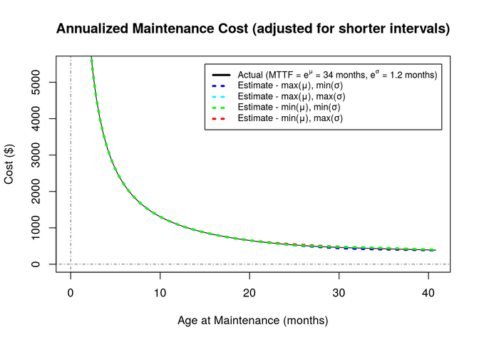
Adjustment Due to Shorter Intervals
Since we are proposing to perform maintenance actions – and incur maintenance costs – prior to pumps actually failing, we need to account for the loss of use of the un-failed portion of the pump's lifetime.
For example, if we simply repaired each pump each week, we would not expect any failures, but we would be paying for 147 weeks (34 months), on average, of repairs. Compare that with paying only one time if we waited for the pump to fail on its own (with no scheduled maintenance).
Remembering the tire analogy, we can think of this as the per-mile cost of the tire, times the number of miles not driven. For the pumps, this is the per-month cost of the maintenance, times the amount of time that the pump is notused.
The amount of time the pump is not used may be estimated by the MTTF value. The per-month cost for the pump is simply the cost of a maintenance event, which is identified in equation (16) as \(C_{\mathrm{maintenance}}\), divided by the interval at which this cost is incurred. We can either compare the per-month costs for all maintenance actions or use some other common time frame.
Since companies typically account for costs annually or quarterly, we can use either of these time frames as a reference. Here, we will use annual costs, so we can simply multiply the monthly cost (maintenance costs divided by the age (in months) at which the maintenance is performed) by 12 (months in a year).
\[\begin{aligned} (17)\quad & C_{\mathrm{adjusted}} = & 12 \, \times \, \left( \frac{C_\mathrm{maintenance}(t_{\mathrm{interval}})}{t_{\mathrm{interval}}} \right) & \quad\text{Annualized cost of early repair} \\ \end{aligned}\]
- # Maintenance costs given maintenance interval
- c_adjusted <- function(t,mu,sigma) { 12 * c_maintenance(t,mu,sigma) / t }
The chart below illustrates this cost and shows that this is the element of cost that penalizes early maintenance with a very high cost for short intervals.
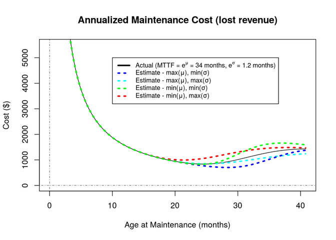
Lost Revenue
The time when a pump is out of service – either for a scheduled maintenance event or for an emergency repair after failure – represents the loss of revenue from that pump. This is considered a cost and must be accounted for when determining the cost of scheduling maintenance for pumps.
In the assumptions, we can see that scheduled outages are much shorter (2 days) than outages due to failures (7 days). This is due to the additional time to detect the failure and schedule the repair. The actual repair time will be the same for both. The revenue lost during an outage is:
\[\begin{aligned} (18)\quad & C_{\mathrm{repair time}}(t) = \frac{\mathrm{Revenue}}{n_{\mathrm{total}}} \, \times \, t & \quad\text{Lost revenue for a repair} \\ & = \, \$782.78 \, \times \, t & \text{[per pump per day]} \\ \end{aligned}\]
The cost of lost revenue for repairing or maintaining a pump depends on the number of repairs after failure(s), and the number of maintenance events prior to failures. This proportion is the quantile that we have used before.
\[\begin{aligned} (19)\quad & C_{\mathrm{lost revenue}} & = q \, C_{\mathrm{repair time}} \left( mttr_{\mathrm{unscheduled}} \right) & \quad\text{Cost due to lost revenue} \\ & & + \left( 1 - q \right) \, C_{\mathrm{repair time}} \left( mttr_{\mathrm{scheduled}} \right) & \\ & & = \$782.78 \, \times \big( 2 \, {\mathrm{days}} \, + \, q \, \left( 5 \, {\mathrm{days}} \right) \big) & \\ \end{aligned}\]
And now we can use the cumulative distribution to translate the formula from the quantiles to the maintenance interval. Since we want to be able to combine this cost with the maintenance cost calculated above, we go ahead and annualize the cost here as well.
\[\begin{aligned} (20)\quad & C_{\mathrm{lost revenue}} & = \frac{12}{t} \, \$782.78 \, \times \big( 2 \, {\mathrm{days}} \, + \, 5 \, {\mathrm{days}} \, \times \, F(t) \big) & \quad\text{Cost due to lost revenue} \\ \end{aligned}\]
- # Maintenance costs given maintenance interval
- c_lostrevenue <- function(t,mu,sigma) { 12 * 782.78 * ( 2 + 5 * plnorm(t,mu,sigma)) / t }
Total Maintenance Cost
Once we have determined the annualized cost to perform the maintenance, and the cost for not having the pumps available during maintenance, we can simply combine the costs to determine the annual cost per pump. This may be compared with the cost of not performing scheduled maintenance, and highlights the benefit of scheduled maintenance. The total cost is the sum of the individual costs:
\[\begin{aligned} (21)\quad & C_{\mathrm{total}} \, = \, & C_{\mathrm{adjusted}} \, + \, C_{\mathrm{lost revenue}} & \quad\text{Total cost per pump} \\ \end{aligned}\]
We can determine the maintenance cost incurred in the absence of any scheduled repairs by setting the maintenance interval to MTTF and the percentage of failed pumps to 100% in the above formulas. The degenerate formulas for no scheduled maintenance are:
\[\begin{aligned} (17a)\quad & C_{\mathrm{adjusted}} \, = \, \$1,360.00 \, \times \, \left( \frac{12}{\mathrm{MTTF}} \right) \, = \, \$480.00 & \quad\text{Annualized cost of repair} \\ \end{aligned}\]
\[\begin{aligned} (19a)\quad & C_{\mathrm{lost revenue}} \, = \, \$782.78 \, \times \, 7 \, = \, \$5,479.46 & \quad\text{Per pump per repair} \\ & \$5,479.46 \, \times \, \left( \frac{12}{\mathrm{MTTF}} \right) \, = \, \$1,933.93 & \quad\text{Annualized} \\ \end{aligned}\]
Resulting in a total cost prior to scheduling maintenance of:
\[\begin{aligned} (22)\quad & C_{\mathrm{total}} \, = & \, \$480.00 \, + \, \$1,933.93 \, = \, \$2,413.03 & \quad\text{Annual cost per pump} \\ & C_{\mathrm{entire}} \, = & \, n_{\mathrm{total}} \, \times \, \$2,413.03 \, = \$16,897,510.00 & \quad\text{Total annualized revenue for repairs} \\ \end{aligned}\]
Now that we have a cost for repairs without schedule maintenance, we can find the cost with scheduled maintenance and then identify the optimum maintenance age for the pumps, as well as the total annualized cost of repairs (to compare scheduled v. non-scheduled).
- total_cost <- function(t,mu,sigma) {
- c_adjusted(t,mu,sigma) + c_lostrevenue(t,mu,sigma)
- }
-
- min_costs <- apply( model_conditions, 1,
- function(r) optimize(total_cost,c(15,mttf),r[1],r[2],tol=0.01))
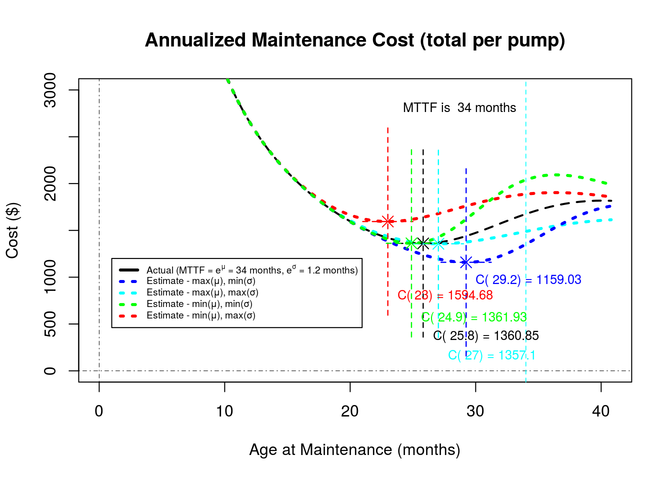
The annualized cost per pump, per year, for the nominal case is $1,360.85. The maintenance interval at the minimum cost (prescribed repair age) is 25.8 months. Annualized and summed over all of the pumps, the cost becomes:
\[\begin{aligned} (23)\quad & C_{\mathrm{total}} \, = & \, \$1,360.85 & \quad\text{Annual cost per pump} \\ & C_{\mathrm{entire}} \, = & \, n_{\mathrm{total}} \, \times \, \$1,360.85 \, = \$9,525,950.00 & \quad\text{Total annualized revenue for repairs} \\ \end{aligned}\]
Discussion and Cautions
To summarize the results:
- When not performing scheduled maintenance (repairing pumps only after failure), the annual cost is $2,413.03 per pump, or $16.9M for the entire business.
- When performing scheduled maintenance at an interval of 25.8 months, the annual cost is $1,360.85 per pump, or $9.5M for the entire business.
- Implementing scheduled maintenance results in a savings of 43.6% (costs are 56.4% of the base case).
- Implementing scheduled maintenance saves $1,052.48 per pump annually, or $7.4M for the corporation.
When we created our model, we made several simplifying assumptions. Among them were that the pumps would fail with a probability described by a log-normal distribution. This may or may not be correct; the actual failure mechanisms that contribute to the failures might generate a different distribution. We did not account for the entire observed failure behavior of real components: which exhibit many failures at an early age - which we ignored assuming the pumps and parts we used were “burned-in”; they also exhibit a small but non-zero failure rate during the majority of their lifetime. We did account for the “end-of-life” failures that are typically observed, but used a log-normal distribution. This is likely to be acceptable, but more detailed analysis is warranted.
Prior to instituting the scheduled maintenance, we would expect to see many failures at a steady rate over time. This would be expected to be near \(\frac{n_{\mathrm{total}}}{\mathrm{MTTF}}\), or 206 failures per month. This would mean that the 50 sample window we assumed for estimating the parameters would span a time of about 1 week.
After adopting the scheduled maintance, we would expect to observe a much smaller number of failures since we are deliberately attempting to perform maintenance prior to failures in most cases. The number of failures that we would expect to see when using scheduled maintenance is \(\frac{n_{\mathrm{total}}}{\mathrm{MTTF}} \, \times \, F(t_{\mathrm{interval}})\) or 13.5 failures per month. This is a much smaller observation rate and a 50 sample window will span a time of 16 weeks. This means that any updates to the maintenance interval will be much slower to adapt to any changes in the actual failure rates if they occur.
From the estimator performance we can see that it is possible to diverge quite far from the actual model parameters for short times. It would be prudent to implement a limit to changes in the maintenance interval in an attempt to smooth any excursions due to estimation error.
From the total cost curve plot, we can see that the area where the optimal maintenance interval occurs is a shallow minimum. This is encouraging since it means that any error in the implemented interval from the actual optimal interval will be close in cost to the desired minimum cost. This means that even if we selected a probability density function that was not accurate, it is likely that a more accurate density function would result in a similar interval selection.
References
For additional Information see the following:
- [1] Dr. Horst Rinne. "The Hazard Rate - Theory and Inference." Department of Economics and Management Science. Justus Leibig University, 2014
http://geb.uni-giessen.de/geb/volltexte/2014/10793/ - [2] R.C. Gupta, S. Lvin. "Reliability Functions of Generalized Log-Normal Model." Department of Mathematics and Statistics. University of Maine, June 2005.
http://www.sciencedirect.com/science/article/pii/S0895717705003511 - [3] Bathtub Curve
https://en.wikipedia.org/wiki/Bathtub_curve - [4] Basics of System Reliability
http://reliawiki.com/index.php/Basics_of_System_Reliability_Analysis - [5] Reliability / Survival Analysis Wiki
https://en.wikipedia.org/wiki/Category:Survival_analysis - [6] Reliability Engineering
https://en.wikipedia.org/wiki/Reliability_engineering - [7] Analyzing Survival or Reliability Data
http://www.mathworks.com/help/stats/examples/analyzing-survival-or-reliability-data.html
Software Engineering Tech Trends (SETT) is a regular publication featuring emerging trends in software engineering.
