Welcome to the Machine (Learning)!
Mike Martinez, OCI Principal Software Engineer
FEBRUARY 2015
Introduction
This article provides a brief overview of machine learning. I will concentrate on aspects of machine learning that apply to almost all strategies for learning: selecting training and validation data and metrics for estimating the suitability of the trained model. And I hope to give you a quick taste of what some of the issues are that you will encounter if you use machine learning as a tool.
Machine learning does not require large amounts of data, but some algorithms and applications do benefit from more data. So machine learning and "Big Data" are associated in many ways. Indeed, some algorithms perform best in the presence of large data sets; processing large amounts of data is a natural application for algorithms that predict outcomes or categorize inputs.
This does not mean that machine learning requires large amounts of data, or that machine learning is restricted to the realm of big data[1]. In some instances, more data is not beneficial and can actually reduce the accuracy of any predictions made by trained models.
The majority of applications for machine learning today, at least those most publicized, involve predictions. These predictions are made by applying new data to a model as the data becomes available.
Models represent the behavior of some external process, which might be a physical process. Models are used to produce outputs that closely match the process being modeled when presented with the same inputs.
Models are constructed by extracting information from training data and using it as parameters that allow the model to closely match the actual output data when given the same input data. The outputs generated from the model are then assumed to be close to what the original process being modeled would have produced given the same inputs.
Stated this way, machine learning is nothing but a computing technique of technical interest. But any practice of machine learning must recognize that the models will be used in a larger context and can have a social impact; either positive or negative.
Some examples of this include the teenager whose pregnancy was deduced by an analytical model before her parents were able to reach the same conclusion. Or, during end-of-year processing some social sites including images of deceased friends and relatives in a celebratory context.
It is good to keep in mind that the use to which models are put is not simply technical.
Overview of Machine Learning
Machine learning grew from work in artificial intelligence and also has close ties to optimization. While there are many definitions of machine learning, here are two that provide a suitable insight from different perspectives into what machine learning is actually about:
A broad definition without much detail:
"Field of study that gives computers the ability to learn without being explicitly programmed."
― Arthur Samuel, 1959[2]
A more thorough definition with, perhaps, too much detail:
"A computer program is said to 'learn' from experience ' with respect to some task 'T' and some performance measure 'P', if its performance on 'T', as measured by 'P' improves with experience 'E'."
― Tom Mitchell, 1998[3]
What these definitions have in common, along with other definitions of machine learning, is that they are describing the use of computers to perform tasks without being programmed for those tasks. This is accomplished by providing data to the software which is then used to determine what behaviors to perform. Indeed, the Tom Mitchell definition can be used as a menu for creating a learning program. Or at least validating that a learning program actually learns.
Machine learning is a very wide ranging topic, and it is easy to get lost in the many different uses and issues with the topic.
A simple way to approach machine learning is to realize that what separates this topic from the usual statistical and analytical topics is the learning.
What is being "learned" is a set of parameters for models which are then used to predict likely outcomes. This vastly oversimplifies what machine learning is, and may exclude some types of learning altogether, but it is a good start.
Machine learning is used to solve problems that otherwise would be too difficult to solve in a useful way. For example, it is possible to match all possible permutations of an image to other stored images in order to do face recognition. But that would likely take longer than acceptable and probably require more processing than is available. Some would argue more time and processing than can be available.
Approaches
The types of machine learning that have been developed are tailored to specific problems. Once a technique for machine learning has been developed, additional problems and applications are then found to which it applies. This happens regularly and machine learning today is a very dynamic topic.
Machine learning solves problems that cannot easily be solved by direct algorithmic approaches. Or which could be solved directly, but not within the constraints of the required solution – such as solving the problem within a given deadline.
A common approach to machine learning software is to collect data of correct input/output relationships generated from some underlying process. Then use an algorithm to create a program to generate the same outputs for these inputs, which is referred to as training. Once trained, the program is then used to process new inputs into new outputs, assuming these outputs are close to what the original process would have produced.
The "program" that is created in the above description typically is a parameterized algorithm that implements one of many different models that are expected to match the original mapping behavior. These models can be from many types, with more being generated or discovered regularly.
Existing models are being tweaked regularly to adjust for known issues as well as new issues as they are discovered. Some of the more well known model types include:
- Regression (linear or logistic)
- Bayes (naive or complex network)
- Neural networks
- Support vector machine (SVM)
- Principal component analysis (PCA)
- Nearest neighbor (k-NN)
- Decision trees
- Random forests
- k-means
- Markov models (HMM)
Problems Solved with Machine Learning
Problems that can be solved using machine learning include almost any problem that can be solved using software. While some problems – such as addition or logical operators – are easier to solve using direct computation or simple algorithms, other problems can only be addressed using a learning approach to be solved within constraints.
A common characteristic of most problems that machine learning addresses is that they are complicated or underspecified. Some problems are large and require either a hierarchical composition of different techniques, an aggregation of techniques, or a complex organization of different techniques in order to achieve a goal. Autonomous vehicles, such as self-driving cars and drones, are an example where many techniques are used to address the different needs of the overall goal.
Some examples of problems addressed by machine learning include:
- Pattern recognition
- Recognizing anomalies
- Prediction
- Data mining
Pattern Recognition
Recognition of patterns can be done in one or more dimensions.
An example of a one-dimensional pattern is the part of speech recognition which involves sampling an audio stream and partitioning it into phonemes.
Two dimensional pattern recognition problems are easily found in image processing, where images are split into relevant regions, or specific objects are located or recognized – such as facial recognition.
Higher dimensional patterns are searched for in multi-spectral and hyperspectral data such as that gathered from satellite imaging.
In addition, natural language processing (NLP) is considered a pattern recognition problem, since it attempts to extract meaning from the patterns of either textual or phoneme based input streams.
Recognizing Anomalies
Anomaly detection is a very important problem being addressed with machine learning. Detection can be used to find spam e-mails and credit card or phone fraud.
Applying machine learning to sensor readings helps detect anomalies in power plant or other critical operations. This can help determine when remedial actions can be taken prior to emergency conditions requiring more drastic measures.
Prediction
Prediction garners the most press for machine learning. It includes applications such as predicting stock price movements, currency exchange rates, and risk analytics &ndash all financial applications of great interest recently.
Politicians can use machine learning for sentiment analysis, and web traffic click-through prediction can help tune commercial web offerings and advertising.
In addition, preferences can be predicted. This use is well known via recommendation engines from providers such as Amazon, Netflix, and others, as well as providing targeted advertisements on web pages.
Data Mining
Historical data can be used to improve decisions. It can also be used to discover unknown relationships in the data. Information retrieval using machine-learning techniques can be used for data mining in many applications, including:
- Genomics
- News/twitter feeds
- Archived data
- Web clicks
- Medical records
This information retrieval is done by finding similar groups of material or summarizing the large input data sets so that they can be categorized and indexed.
Types of Machine Learning
There are three main types of machine learning:
- Supervised
- Unsupervised
- Reinforcement
Each of these types is suitable for solving different problems, so each type is undergoing research and development.
In addition to these types of learning, aggregation of multiple models is sometimes used to create an overall model with better performance than any of the individual models provide when used alone.
Supervised Learning
Supervised learning is typically used to predict output values given input values. Classification problems – binary and multi-class categorizations – are solved well using models trained using supervised learning techniques. Continuous valued problems are also solved using supervised learning models.
Supervised learning configures a parameterized model with values obtained from a training process. The training process uses input values along with the known desired result matching those input values. These input/output sets are used to derive model parameters that allow the model to match the actual training data as closely as possible.
Selection of the model, or algorithm, determines not only what the parameters are that need to be determined, but the possible solutions that can be modeled using that technique.
For example, if a linear model is used to estimate a quadratic process, no parameter value assignments will be able to reduce errors enough to make a useful prediction.
Once a model has been selected, then the parameters must be determined. Supervised machine learning does this by successively presenting individual training input/output sets and adjusting the model parameters to minimize the measured error.
This means that there must be an algorithm for adjusting the parameters as well as a formula for measuring the error. A gradient descent algorithm – one that changes parameters in a direction and amount towards smaller errors – is commonly used to adjust the parameters. But other optimization techniques can be used as well. The measurement of error is performed using what is called a "cost" function.
Model types that are used for supervised learning include decision tree models, regression models, and neural networks, among many others. All of these models are characterized by having a simple structure with enough parameters to provide a complex transfer characteristic between the inputs and outputs. This allows the parameters to be adjusted to match many types of external processes being modeled.
One supervised learning model of special note is the "k nearest neighbors (k–NN)" model. This is a supervised learning model since it uses training data to extract model parameters. What makes this model unique is that training is instantaneous, since the model parameters are defined to be the training data.
For classification use, this model type simply finds the k nearest training data points to the input data and uses them to vote on the input category. For continuous valued (regression) use, the output can be an average of those nearest parameter points – effectively a multi-dimensional interpolation.
Unsupervised Learning
Unsupervised learning is used to discover a good internal representation of the input data.
This style of machine learning was not considered machine learning at first, since it does not have an explicit training technique. It can be difficult to determine what the actual goal of unsupervised learning is.
Some applications for this type of machine learning include creation of a model or representation that can subsequently be used for supervised learning.
Unsupervised learning extracts model parameters from input data without having any desired – or correct – output values with which to train the model. This means that the optimization techniques used with supervised learning cannot be used, since a cost function cannot be created.
Unsupervised techniques used include dimensionality reduction, such as Principal Component Analysis (PCA), and clustering, such as k-means. These techniques can derive a model that characterizes the inputs, determining clusters of similar inputs or extracting the most important features of the input data.
Once the features have been extracted, they can then be used for subsequent supervised learning if desired.
A problem with the models based on extracted features is that the features rarely correspond to describable features. For example, when clustering phone customers into those that leave a provider and those that do not, the combination of input factors used to create the features may not have any discernible reason. So while the model may accurately predict if a customer will leave the provider, no underlying reason can be identified.
Reinforcement Learning
Reinforcement learning is used to select actions that maximize a payoff. What actions are, and what payoffs are, are determined when framing the problem to be solved.
This type of learning is able to make decisions in an attempt to optimize an end result. The techniques lend themselves well to operation in a changing environment, since each decision is made within the context existing at the time.
Reinforcement learning uses a heuristic function to calculate a cost for each of many possible actions and selects the action with the smallest cost. The selection of a heuristic function is critical to these algorithms. Discounting can be applied within the heuristic in order to minimize the effect of conditions far removed (in the far future) on current decisions.
The path-finding A-star algorithm is a reinforcement learning algorithm. In addition Monte Carlo simulations, optimal control, and error driven algorithms are used for reinforcement learning.
Some examples of problems solved using reinforcement learning include route planning, activity planning, puzzle solving, robotics, and resource allocation. Resource allocation can be especially dynamic – when dispatching emergency services during on ongoing disaster, for example.
Reinforcement learning does not establish a fixed model and use it on subsequent inputs; it calculates costs at each decision point. This makes it robust in changing environments. Allowing dynamic adjustments to the heuristic function even allows the ultimate goal of a model to be changed during operation.
For example, when calculating a route from home to work, costs can be determined using the current traffic conditions. But once traffic conditions change, subsequent decisions can be based on the new information rather than the original conditions. And the addition of an extra waypoint can be accommodated at any time.
Reinforcement learning can be difficult for many reasons. These include heuristic function selection, delayed payoffs, unknown critical decision points, and a changing environment. Many difficulties derive from the characteristic of the cost value generated by the heuristic function being a scalar which can not encode detailed information about goals or costs.
Model Aggregation
In addition to the above learning types, combining multiple models to operate over the same inputs can produce better predictive performance that any single model alone.
There are many ways to aggregate more than one model. These include:
- Bootstrap (bagging)
- Boosting
- Bayesian techniques
- Stacking
The aggregated models are trained together as if they were a single model, with an aggregate cost function used for optimization.
Typically fast algorithms, such as decision trees, are used for aggregated models, but even slow algorithms can benefit.
Bagging collects the results from many models and combines them with equal weight. Random forests are an example of this, where many decision tree models are executed and the output averaged. Bagging can suffer from overfitting or underfitting of the training data, depending on the problem being solved. Unfortunately it is not easy to tell which, if either, of these problems may be encountered.
Boosting incrementally builds a collection of models by training each model based on the result of previous model training. This is more likely to overfit data than individual models. But the improved accuracy makes the technique worthwhile.
Bayesian techniques include optimal (which is not practical), averaging, and combining. The averaging technique attempts to approximate the optimal results, and combining is an algorithmic modification of the averaging algorithm. Cross validation results are used to determine the final result for these techniques.
Data
Machine learning requires data. How that data is obtained is not relevant to the training or predictions of the models created through machine learning. But the quality and amount of available data may constrain what models are possible to use for predictions.
For some data, such as that generated within an internet environment, it is easy to gather data in any amount, and quality can be used as a criterion for what data to select. Other data, such as medical data from a longitudinal study over decades will not only be small in size, but it would be very difficult to create more.
The amount of data required will be driven by both how accurate the performance metrics will need to be, as well as how the selected model training performance improves with data size. Once a candidate amount of test data (used to measure model performance) and training data (used to extract model parameters) is selected, the total amount of data required can be established.
Once a dataset has been acquired, it should be partitioned into three sets of data, each with a different purpose:
- Test data
- Cross validation data
- Training data
The first data to extract from the available data should be the test data.
This typically consists of 10% to 20% of the total available data and should never be seen by the prediction model during training or validation. The only time this data should be presented to the model is during testing to evaluate trained model performance.
Data extracted for testing and training should always be drawn from the same population; i.e., training with one dataset then using a different dataset to test with should not be done.
Once a model has been trained, additional data – cross validation data – is used to measure the performance of the model.
Additional steps can then be taken to modify the model and improve performance. Typically about 20% of the original data is reserved for cross validation. What remains of the original data (about 60% – 80%) after removing the test data and the cross validation data is what will be used for training.
Some cross validation techniques repeatedly resample the training and validation sets to generate many different training and validation passes through the data. Each time the data is sampled, it should be done randomly. If feature selection or model tuning is required for training, such as PCA parameter mapping, then this must be done for each training set that is extracted.
When working with time series data, such as stock prices or weather data, contiguous subsequences should be extracted from the data, with each subsequence being selected randomly.
Depending on the details of training, overlapping of sequences may or may not be allowed. If no overlap is allowed, then a very large amount of data must be available or fewer validation sets extracted.
Training Algorithm
Training is how model parameters are optimized to match the desired input/output transformations as closely as possible.
This is an extensively studied topic for optimization and many possible solutions are available. The most prevalent technique is to use the gradient descent algorithm to find the lowest error between a model and what it is modeling.
Optimization is performed by minimizing a cost function over all possible parameter values. For machine learning, the parameters correspond to model parameters. The cost function is the measured error, as a scalar, between the model and the process being modeled. Gradient descent uses the following algorithm:
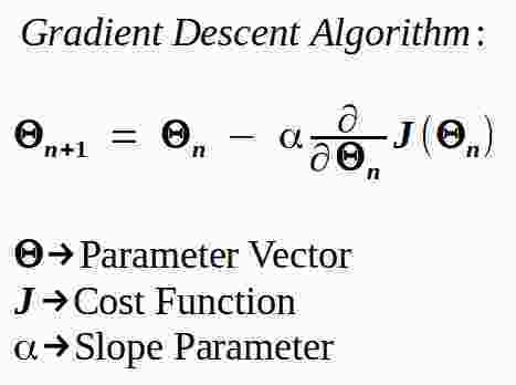
Where the parameter vector includes all of the model parameters being adjusted, with the next values of the parameters generated from the current values of the parameters, the adjustment is a scaled value of the gradient of the cost function for the current values.
Cost functions measure the model's "goodness of fit" to the actual data.
This is easily done by generating a prediction from the model for input values and comparing the result with the actual expected value. This is what a single calculation does during training – it uses the current parameter values to generate a predicted value for the input data then determines an error based on the predicted and expected values.
A cost value commonly used is the average of the squared error (distance between the desired and predicted values).
Cost functions can be simple or complex. Gradient descent is most useful for simple cost functions.
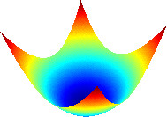
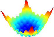
The diagrams below show possible cost functions for a two parameter model. The parameters are represented by the x and y axes with the cost function value represented as the z axis value.
The simple surface is smooth and you can see that moving towards a lower cost will always reach the globally optimum value.
The complex surface is not smooth and contains many local minima. Simply following the direction of lower cost from any point will more likely find the nearest local minima rather that the global minimum. This is the optimization problem that needs to be solved.
A good solution to the problem of becoming stuck in local minima is to craft a cost function that is smooth, if possible.
Cost Surfaces for Optimization
Simple
Complex
The slope parameter in the gradient descent formula is also known as the learning rate (α) coefficient. It determines how quickly the solution is reached.
Small values of α will cause small steps between successive parameter estimates. This means that convergence to a final value will take longer. Larger values of α will take larger steps, but also may cause the algorithm to become unstable and not converge at all.
Typically values less than 1 are used to avoid instabilities. Modern algorithms will update the learning rate adaptively to ensure convergence as well as complete quickly.
Parameter values obtained from the learning algorithm can be measured using the test data. Since the test data has never been seen by the model previously, the performance of the model for this data gives us confidence that the model will work on novel input data. If the performance of the model for the input data matches the performance on the training data, then the model is considered a good fit.
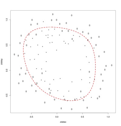
The diagram below shows a classification boundary for a model with a good fit. The diagram plots each input using the values of the two parameters for that input set. The symbol used (o or +) indicates the correct output classification. The red boundary shows where the model switches predictions of the output value for the given parameter values. The two classifications are separated from each other by the boundary with just a few points mis-classified.
Good Fit
λ = 1.0
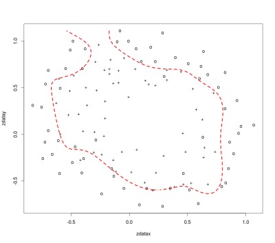
It is possible to create a boundary that too closely fits the training data – overfitting.
This means that the model can achieve up to perfect performance for the training data, but performance for data sets other than the training data is much lower. This can happen when a complex model is used to fit noisy data for a simple process. The trained model will be complex enough to correctly classify the training set, but the boundary will be specific to that data, and new data is likely to be mis-classified.
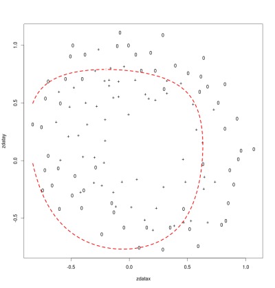
Another problem can occur when the model does not perform well on the training data or the test data. This is known as underfitting.
These models are simply not good enough to use for new input data. The diagrams below illustrate what an overfit and underfit model can look like for a prediction model similar to the one shown above with a good fit. You can see that the overfit model traces a boundary around points within the training data. The under fit model simply gets the boundary in the wrong location.
Over Fit
λ = 0
Under Fit
λ = 20.0
One approach to avoid overfitting the training data is to add a smoothing parameter to the cost function. For regression models, this can simply be the addition of a term that includes the sum of all the squared parameter values. This term is conditioned with a scale factor commonly named λ.
The smoothing of the cost surface is known as regularization. A λ value of zero corresponds to the original cost function. This will lead to overfitting if models are too complex for the underlying modeled process.
λ values greater than one lead to underfitting since it tends to drive all parameters to a similar value. A value near one will limit the magnitude of individual parameters without distorting the overall model.
The diagrams above use the same model and parameters, but were trained with the values of λ shown.
Cross Validation
Cross validation (known as rotation estimation to statisticians) is a technique that estimates how the trained model will generalize to independent input data. This allows us to estimate how the model will perform on new data using only the training and validation data we have.
Techniques for cross validation consist of generating many training and validation sets from the available data. The results from training and validating for each partition can be combined to give a better estimate of the expected model performance. For some models, the results can be used to adjust the parameters to get better overall performance. It is also possible to compare different error metrics or the suitability of different models to a problem using cross validation.
Partitioning the data into training and validation sets can be done in different ways. It may be impossible to exhaustively calculate all training and validation sets if the number of generated data subsets grows large. Mechanisms for cross validation commonly used include: leave-p-out, k-fold, and random sub-sampling. leave-1-out and 2-fold cross validation are special cases of the above that are more simply implemented.
The leave-p-out cross validation procedures consist of repeatedly selecting p data elements for validation with the remaining data elements used for training. This is then done for each possible combination of p elements. This suffers from a combinatorial number of trials to execute for non-trivial p but degenerates into a number of trials equal to the data set size for the special case where p is 1.
The k-fold cross validation procedure consists of partitioning the dataset into k equal pieces ― the folds ― then sequentially using each of the k partitions as the validation data with the remaining data as the training data. A common value of k is 10. If the value is equal to the number of data elements, then this is identical to the leave-1-out cross validation. One specialization of this technique, stratification, is to partition the dataset into the k subsets such that the average response for each subset is approximately the same. Note that this technique also ensures that each data element is used for both training and validation. Each data element will be used only once for validation.
2-fold cross validation is a specific version of k-fold validation where the data is partitioned into 2 equal sets and each set is used once for training and once for validation. This ensures the largest equal size of training and validation data as well as the use of each data element once in each role.
It is also possible to simply generate a sequence of random subsets of the data and perform sequential training and validation on each subset. This means that the proportion of training to validation data is not constrained by the number of folds. But it is also likely that the validation subsets will overlap and that some data will never be included in a validation subset.
Machine Learning Metrics
Performance of machine learning is based on several metrics. These metrics attempt to characterize the difference between predicted values and actual values. When the two are close, the performance is considered better than when they are not close.
Sources of errors that affect performance include bias, variance, and noise. Measures of performance include mean-squared error for continuous models and those based on the confusion matrix for classification models.
Errors
Sources of error in model performance can be separated into three different categories: bias, variance, and irreducible errors.
Bias is error introduced by algorithmic or model errors.
Variance is variability in model predictions for a given data point, or the sensitivity of the model to the data.
Irreducible errors are noise that cannot be removed from the model or the data.
Bias Errors
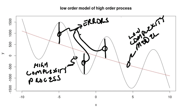
Bias errors are a measure of the match, or suitability, of a model to be used for predicting an actual process. If the process being estimated is more complex than the model, the model will never be able to predict the outcomes of the process with any accuracy.
Bias error can be reduced by making a model more complex (adding additional parameters) but will not be reduced by adding more data to the training set.
In the diagram below, a complex process is represented by the oscillating curve. If a simple linear model is used to predict the outcomes of the process, it will not be possible to minimize the error since the model will always be some distance from the actual values of the process.
You can see intuitively that making the model more complex – able to include more detail, or curves – will allow the model to more closely fit the process being modeled. You should also be able to see intuitively that adding more data to the training set will not affect the performance of the model.
High Bias Model Fit
Variance Errors
Variance errors are due to model sensitivity to data.
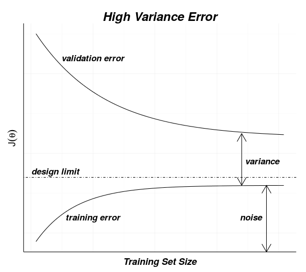
As models become more complex, variance errors tend to increase. As more training data is added, the variance errors tend to decrease.
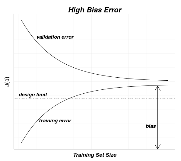
The diagram below shows curves for measured errors for training and validation data sets for a model. As the training (or validation) size increases, you can see that the training error increases to a point that includes the noise error. The validation measurements drop from a larger value towards the training error.
This behavior can be understood by recalling that during training, each subsequent input element adds more data for the model to fit.
The very first training data element will have no error since there is only one set of data to fit. After that it becomes more difficult to fit the model to the data. If the model is suitable, then after the entire training data set has been presented, the model will have only noise error between the predictions and the actual values.
For the validation data, it is unlikely that the first value will be close to the model for a single data element. As more elements are used to train the model, the validation data should approach the residual error of the training data.
The difference between the expectation (noise error residual for the training data curve and the validation data error matching the training data error) and measurements then is how we can recognize the bias and variance errors.
If there is high variance, the asymptotes which the top and bottom curves approach are far apart. Adding more data should bring these closer – reducing variance errors – since the slope of the top curve continues towards the bottom curve.
If the two curves approach closely but the residual error is high, that indicates that there is a high bias error for the model. Adding more data will not change the bias error. More data will only bring the curves closer without changing the asymptotic value they are approaching.
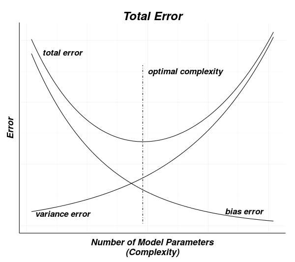
It is tempting to make models very complex to reduce bias errors as much as possible.
This is not a good strategy since bias errors and variance errors work in opposition. That is, as models become more complex (more parameters to fit), the variance error will increase as the bias error decreases.
The optimal solution is to find where the combination of these effects produces the overall minimum error. An intuition for this process can be seen in the next diagram.
Classification Performance
For measuring classification performance, a confusion matrix is used. This is also known as a contingency table. This table is well known in statistics to show where type I and type II errors occur for binary classification.
The confusion matrix can be extended to include performance for more than two categories, but I will discuss just the simple binary categorization case here.
The confusion matrix typically has the actual values as the columns of the x axis, and the predicted values as the rows of the y axis. This gives the for cell table as below:
When measuring a model's performance, each predicted result should be added to one of the cells in the matrix. Once all of the data to be measured has been entered into the table, then row and column sums can be formed, and additional measurements derived from this data. Some of the common metrics include accuracy, precision, sensitivity, and specificity.
Each metric gives an indication of the model performance for a particular characteristic.
All of the metrics should be considered when evaluating model performance. Some metrics become more important as the matrix becomes less balanced.
For example, if we have a process where there are few positives – such as fraud detections – then metrics such as accuracy will be high even with a poor model.
If true fraud rates are at 1%, then predicting no fraud always will have an accuracy of 99%, which may give a false confidence for a model that would fail to detect any fraud.
The list below summarizes some of the more common metrics that can be derived from the confusion matrix:
| Measure | Formula | Description |
|---|---|---|
| Accuracy | (TP+TN) / (TP+FP+TN+FN) | overall rate of correct predictions |
| Precision (Positive Predictive Value – PPV) |
TP / (TP+FP) | accuracy of true predictions |
| Sensitivity (True Positive Rate – TPR) |
TP / (TP+FN) | rate of true predictions for true values |
| Specificity – SPC (True Negative Rate – TNR) |
TN / (TN+FP) | rate of false predictions for false values |
| Negative Predictive Value – NPV | TN / (TN+FN) | accuracy of false predictions |
| False Discovery Rate – FDR | FP / (FP+TP) | inaccuracy of true predictions |
| False Negative Rate – FNR Miss Rate |
FN / (FN+TP) | rate of false predictions for true values |
| False Positive Rate – FPR Fallout |
FP / (FP+TN) | rate of true predictions for false values |
Some sources will name the metrics slightly differently, so it is good practice to check metric formulas to ensure that you understand which measures are being reported.
There are more possible metrics that can be derived from the table, but the above set should be sufficient to characterize a model.
Try it!
If you want some hands-on experience with machine learning, I highly recommend Andrew Ng's Machine Learning[4], a Stanford course presented through the Coursera MOOC.
In order to demonstrate some of the concepts we discussed, I created a Shiny application[5] that implements a machine learning algorithm in the R language.
If the server is not responsive for the application included inline below, you can obtain the application from GitHub[6] and run it locally using RStudio.
The Shiny Application
This application implements classification by implementing a prediction model using logistic regression for two categories.
I generated a random data set to work with that should result in a mostly circular boundary for the categories. This data represents a binary classification for a two parameter model.
The data is classified into one of two categories and shown in the diagrams as either a '+' or 'o' symbol. A linear optimization routine is provided the cost function and its derivative function (recall that the derivative is the gradient used for modifying parameters).
The R code for the cost function and derivative functions used are shown below.
The Shiny application contains adjustments to several parameters for the model and training. These include:
- lambda, the regularization parameter
- complexity, a measure of the number of model parameters
- maximum iterations, a stopping condition for the optimization
- contour gridlines, setting the accuracy of the plotted classification boundary
- threshold, the plotted boundary for predictions from the model.
The logistic regression cost function and gradient implemented are defined in the formulas below.
The formulas assume there are m data elements, using subscript i, and n parameters with subscript j.
The model is represented by the hypothesis function h which is a sigmoid transformation of the polynomial in the input variables that can be modified to adjust the complexity of the model.
Cost and Gradient Functions for Logistic Regression

- #
- # Generate the sigmoid transformation of input data.
- #
- sigmoid <- function(x) 1 / (1 + exp( -x))
-
- #
- # Cost function
- #
- # theta - p x 1 matrix of parameters to optimize
- # x - m x p matrix of data to train with
- # y - m x 1 matrix of classification values for training
- # l - regularization scaling factor
- #
- reglogregJ <- function(theta, x, y, l) {
- # scalar - number of training data elements
- m <- length(y)
-
- # m x 1 matrix - hypothesis function values for the training data
- h_theta <- sigmoid(x %*% theta)
-
- # m x 1 matrix - cost values for each training data element
- terms <- -y * as.numeric(log(h_theta)) - (1 - y) * as.numeric( log(1 - h_theta))
-
- # p x 1 matrix - parameters with 0 bias term
- nobias <- rbind(0,as.matrix(theta[2:length(theta)]))
-
- # scalar - regularization constant for the parameters
- reg <- l * sum(nobias^2) / (2*m)
-
- # scalar - cost of the current parameter values
- J <- reg + sum(terms) / m
- }
-
- #
- # Cost function gradient
- #
- # theta - p x 1 matrix of parameters to optimize
- # x - m x p matrix of data to train with
- # y - m x 1 matrix of classification values for training
- # l - regularization scaling factor
- #
- reglogregGrad <- function(theta, x, y, l) {
- # scalar - number of training data elements
- m <- length(y)
-
- # p x 1 matrix - parameters with 0 bias term
- nobias <- rbind(0,as.matrix(theta[2:length(theta)]))
-
- # m x 1 matrix - hypothesis function values for the training data
- h_theta <- as.numeric( sigmoid(x %*% theta) )
-
- # p x 1 matrix - regularized gradients for each parameter
- grad <- (colSums(apply(x,2,'*',(h_theta - y))) + l * nobias) / m
- }
The complexity of the model can be set to between 1 and 17. This is a measure of the degree of the parameters used for the model.
A polynomial in the two data parameters up to that degree is generated, with a model parameter for each term in the two variables for all possible combinations of powers. So a degree of 1 would create a model with p0 + p1*X + p2*Y, and a degree of 2 would generate a model with p0 + p1*X^2 + p2*X^2Y + p3*X^2Y^2 + p4*X + p5*XY + p6*XY^2 + p7*Y + p8*Y^2.
The code below shows the function that expands the input dataset into a more complex model determined by the complexity value.
- #
- # Augment a set of points with a bias term and polynomial features up to the
- # specified degree.
- #
- expandFeatures <- function( points, degree=6) {
- result <- matrix(1,dim(points)[1],1)
- for(outer in 1:degree) {
- for(inner in 0:outer) {
- result <- cbind(result,points[,1]^(outer-inner) * points[,2]^inner)
- }
- }
- result
- }
Note that plotting can take a long time, since it is computing a predicted value for each of the grid points.
The default gridlines parameter of 100 will cause 10,000 predictions to be generated and then plotted. For this reason, you should probably adjust the parameters to reach a desired condition and then plot the result.
Summary
We covered a lot of ground here – from problems that can be solved to measuring solution performance to the importance of selecting training data, selecting the right algorithm, validating the training, testing, and measuring performance.
My hope is that you will be able to follow more writing on the subject now, or at least understand the vocabulary being used in order to determine if a particular application or solution is a fit for a problem you need to solve.
There are many additional techniques and methods that need to be applied to any machine-learning application, but they will all likely start with the basics we covered here.
All techniques will be improved with additional measurement at all points during the lifetime of an application. If conditions change while an application is fielded, then additional training (retraining) may be necessary. If the characteristics of the system being modeled change, then selection of a more appropriate algorithm may become necessary.
Steps to create a working prediction model using machine learning will likely include the following steps:
- Describe the problem
- Select a candidate solution
- Select an algorithm
- Obtain data
- Partition the data
- Train the algorithm
- Validate the training
- Measure performance
- Test the solution
- Measure performance
- Deploy the application
- Monitor the performance
References
- [1] Data versus Theory
http://technocalifornia.blogspot.com/2012/07/more-data-or-better-models.html - [2] Phil Simon, p89
https://books.google.com/books?id=1ekYIAoEBrEC - [3] Tom Mitchell, p2
https://books.google.com/books?isbn=0070428077 - [4] Machine Learning, Andrew Ng, Stanford
https://www.coursera.org/course/ml - [5] Demonstration Shiny application
https://objectcomputing.shinyapps.io/settFeb2015/ - [6] GitHub project for Shiny application
https://github.com/brillozon/sett-1502-logisticfit.git
Software Engineering Tech Trends (SETT) is a regular publication featuring emerging trends in software engineering.
